CAD Data Encoding

Table of Contents

Overview

What is CAD Encoding?

The CAD Encoding module (hoops_ai.cadencoder) is the bridge between CAD geometry and machine learning. It transforms symbolic CAD representations (surfaces, curves, topological relationships) into numeric feature vectors that neural networks can process.

Tip

New to CAD or ML? This guide assumes familiarity with:

• CAD concepts: B-rep, Topology, faces, edges → See CAD Fundamentals

• ML concepts: Feature vectors, graph neural networks, node features → See Machine Learning Fundamentals

• Key terms: Check the Glossary for quick definitions

The Core Challenge:

CAD files store geometry in a semantic, mathematical form (symbolic representations with precise meaning):

• A planar face is stored as: “Plane equation: \(0.707x + 0.707y + 0z = 10\)”

• A cylindrical face is: “Cylinder with axis \([0, 0, 1]\), radius \(5mm\)”

• Face adjacency is: “Face #5 and Face #12 share edge #23”

Machine learning models need fixed-size numeric vectors (feature vectors - arrays of numbers representing object properties):

• Face features: [area, perimeter, centroid_x, centroid_y, centroid_z, ...]

• Edge features: [length, angle, curvature, ...]

• Graph structure: edges = [[src_nodes], [dst_nodes]]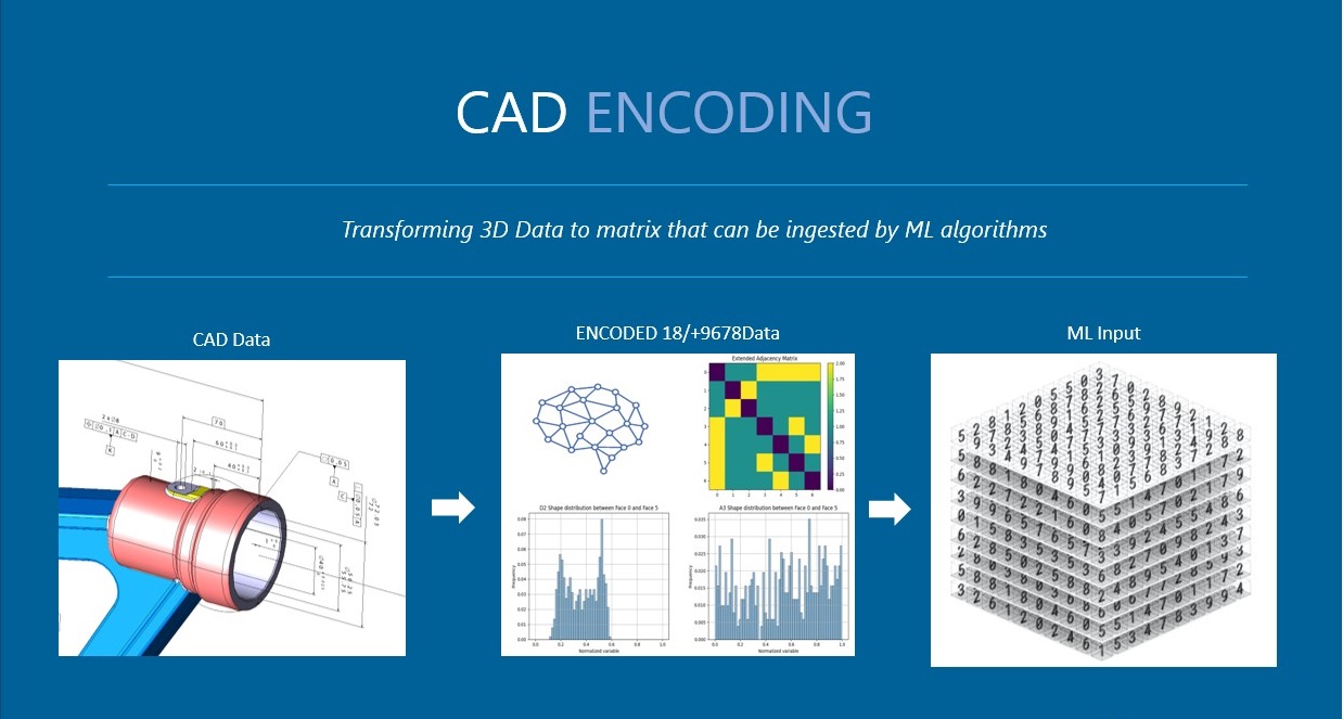

What This Module Does:

hoops_ai.cadencoder provides the BrepEncoder class that:

1. Queries CAD data using HOOPSBrep interface (from cadaccess module)

2. Computes numeric features (areas, lengths, angles, surface types)

3. Structures data for ML (face adjacency graphs, feature arrays, UV grids)

4. Persists to storage using DataStorage interface (from storage module)

Why “Push” Methods?

The BrepEncoder class computes and persists geometric and topological features from BREP data. It follows a push-based architecture where each method:

1. Checks if data already exists in storage

2. Ensures the appropriate schema definition exists for the data

3. Computes the feature if needed

4. Saves to storage with schema management

5. Returns None (if storage is used) or the computed data (if no storage)

The encoder automatically manages schemas for data organization, creating groups and arrays as needed during the encoding process.

See also

• CAD Data Access - How to query CAD geometry using HOOPSBrep

• Data Storage - How DataStorage works and when to use different backends

• CAD Fundamentals - Understanding B-rep topology and geometry

Architecture - How Encoding Works

The Data Flow:

CAD File (part.step)
      ↓
HOOPSLoader (loads file)
      ↓
HOOPSModel (in-memory representation)
      ↓
HOOPSBrep (query interface)
      ↓
BrepEncoder ←--------→ DataStorage
(feature extraction)  (persistence)
      ↓
Encoded Dataset (.data file or memory dict)

Component Interaction:

1. HOOPSBrep: Provides query methods (get_face_attributes(), get_edge_attributes(), build_face_adjacency_graph(), etc.)

2. BrepEncoder: Orchestrates feature extraction by calling HOOPSBrep methods

3. DataStorage: Receives extracted features and saves them (Zarr arrays, JSON, etc.)

Why This Architecture?:

• Separation of Concerns: HOOPSBrep focuses on queries, BrepEncoder on feature engineering, DataStorage on persistence

• Testability: Mock HOOPSBrep and DataStorage for unit testing encoders

• Flexibility: Swap storage backends without changing encoding logic

Tip

Getting Started? If you’re new to this workflow:

1. Start with the simple example in the next section

2. See Tutorials for hands-on encoding walkthroughs

3. Understand what gets encoded by reading CAD Fundamentals first

The BrepEncoder Class

What is BrepEncoder?

BrepEncoder is the main feature extraction engine in HOOPS AI. It systematically processes a B-rep model and generates all the numeric features needed for ML training.

Initialization:

from hoops_ai.cadencoder import BrepEncoder
from hoops_ai.storage import DataStorage

# With storage
storage = DataStorage(...)
encoder = BrepEncoder(brep_access=brep, storage_handler=storage)

# Without storage (returns raw data)
encoder = BrepEncoder(brep_access=brep)

Parameters:

• brep_access (HOOPSBrep): BREP interface from a loaded CAD model

• storage_handler (DataStorage, optional): Storage backend for persistence

Constructor Signature:

def __init__(self, brep_access: HOOPSBrep, storage_handler: DataStorage = None):
   """
   Args:
      brep_access: The B-Rep geometry data source interface (from cadaccess module)
      storage_handler: Optional, object to load/save data from disk or memory
   """

What the Encoder Needs:

• A hoops_ai.cadaccess.hoops_exchange.hoops_brep.HOOPSBrep object (from loaded CAD model) - this is the “source” of geometric queries

• Optional hoops_ai.storage.DataStorage object - this is the “sink” where features are saved (if None, methods return data directly)

Note

Prerequisite: Understand what face adjacency graphs are and why they matter. See:

• CAD Fundamentals - B-rep Topology section explains faces, edges, adjacency

• CAD Data Access - Topological Queries section shows how to build adjacency graphs

Topology Encoding Methods

What is Topology Encoding?

Topology encoding extracts the connectivity structure of the B-rep - which entities connect to which. This is distinct from geometry encoding (sizes, shapes, positions). See CAD Fundamentals for the difference between Topology and geometry.

Why Topology Matters for ML:

• Graph Neural Networks: Topology defines the graph edges (Message Passing paths) - see Machine Learning Fundamentals for how GNNs use graph structure

• Feature Recognition: Machining features are subgraphs with specific topology (e.g., “pocket = 6 connected planar faces forming a box”)

• Manufacturing Constraints: Adjacent faces must have compatible machining directions

• Segmentation: Group faces that are topologically connected

BrepEncoder.push_face_adjacency_graph()

The method BrepEncoder.push_face_adjacency_graph builds a face adjacency graph from the B-rep model. This graph represents the topology of the model where nodes are faces and edges connect adjacent faces.

What It Does:

Build a graph representation of face connectivity where faces are nodes and edges represent shared boundaries.

Mathematical Formulation:

Define an undirected graph \(G=(V,E)\) where:

\[ \begin{align}\begin{aligned}V = \mathcal{F} = \{f_0, f_1, \ldots, f_{N_f-1}\}\\E = \{(f_i, f_j) : f_i \text{ and } f_j \text{ share an edge}\}\end{aligned}\end{align} \]

The graph is represented by:

• Node count: \(|V| = N_f\)

• Edge list: \(\{(s_k, d_k)\}_{k=0}^{|E|-1}\) where \(s_k, d_k \in V\)

Method Signature:

def push_face_adjacency_graph(self) -> Union[Tuple[str, int, int], nx.Graph]:
   """
   Returns:
      If storage_handler is not None:
            Tuple[str, int, int] - (storage_key, num_faces, num_edges)
      If storage_handler is None:
            nx.Graph - the face adjacency graph directly
   """

Usage:

# we assume 'cad_model' is your loaded CADModel instance
from hoops_ai.cadencoder import BrepEncoder
brep_encoder = BrepEncoder(cad_model.get_brep())

adj_graph = brep_encoder.push_face_adjacency_graph()
print(adj_graph)

import networkx as nx
import matplotlib.pyplot as plt

pos = nx.spring_layout(adj_graph)               # compute layout once
nx.draw_networkx(adj_graph, pos, arrows=False)   # draw nodes, edges, labels
plt.axis('off')                         # turn off axes for clarity
plt.show()

Example Output:

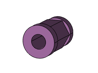
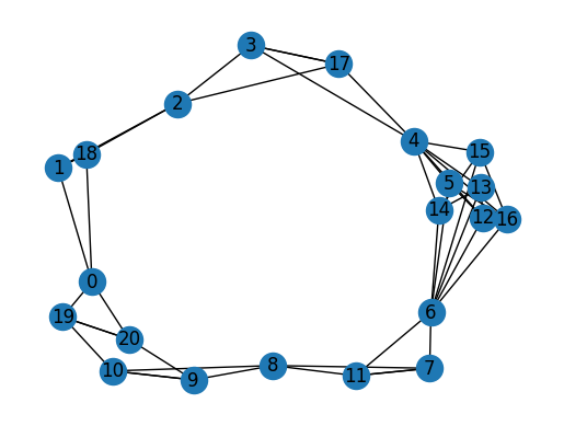
This example shows a DiGraph with 21 nodes and 46 edges. The images below show the 3D CAD model and its corresponding face adjacency graph:

3D CAD model with 21 faces

Face adjacency graph representation

The graph visualization shows nodes (faces) numbered 0-20 and edges connecting adjacent faces. The spring layout algorithm positions the nodes for clarity. Each node in the graph corresponds to a face in the 3D model, and edges represent shared boundaries between faces.

Storage Format Details:

The encoder stores graph data in two formats simultaneously for compatibility:

1. Flat arrays:

   • num_nodes: scalar count of nodes in the graph

   • edges_source: source node indices for each edge

   • edges_destination: destination node indices for each edge

   • graph: nested structure containing edges dict and num_nodes (for backward compatibility)

2. Nested dictionary: Dtypes: int32

Returns:

• With storage: Returns None (data is stored with keys: “num_nodes”, “edges_source”, “edges_destination”, and “graph”)

• Without storage: Returns nx.Graph - NetworkX graph object with edge attributes

Note

Understanding the format: If you’re unfamiliar with graph representations for ML, see Machine Learning Fundamentals - the “Graph Representation of CAD Models” section explains nodes, edges, and node features.

BrepEncoder.push_extended_adjacency()

The method BrepEncoder.push_extended_adjacency computes the extended adjacency matrix representing shortest path distances between all pairs of faces and ensures ‘extended_adjacency’ is in storage or returns the extended adjacency data directly.

What It Does:

Computes shortest path distances between all pairs of faces using Floyd-Warshall algorithm on the face adjacency graph. This provides global topological context.

Method Signature:

def push_extended_adjacency(self) -> Union[str, np.ndarray]:
    """
    Returns:
        If storage_handler is not None: str - storage key ("extended_adjacency")
        If storage_handler is None: np.ndarray - shape (num_faces, num_faces)
    """

Usage:

# Compute all-pairs shortest paths
key = encoder.push_extended_adjacency()

# Later: check topological distance
distances = storage.load_data("extended_adjacency")
# distances[i, j] = shortest path length from face i to face j
# distances[i, i] = 0 (same face)
# distances[i, j] = 1 (directly adjacent)
# distances[i, j] = 2 (connected through one intermediate face)

Mathematical Formulation:

Compute the graph distance matrix \(\mathbf{D}_G \in \mathbb{R}^{N_f \times N_f}\):

\[\begin{split}D_G[i,j] = \begin{cases} 0 & \text{if } i = j \\ \min\{|p| : p \text{ is path from } f_i \text{ to } f_j\} & \text{if path exists} \\ \infty & \text{otherwise} \end{cases}\end{split}\]

where \(|p|\) is the number of edges in path \(p\).

This is computed using the Floyd-Warshall or BFS algorithm via NetworkX’s all_pairs_shortest_path_length.

Storage:

• Array: extended_adjacency

• Shape: [node_i, node_j]

• Dtype: float32

Returns:

• With storage: Returns None (data is stored with key "extended_adjacency")

• Without storage: np.ndarray of shape (N_f, N_f)

BrepEncoder.push_face_neighbors_count()

The method BrepEncoder.push_face_neighbors_count counts the number of adjacent faces for each face and ensures ‘face_neighborscount’ is in storage or returns the neighbor counts directly.

What It Does:

Count the number of adjacent faces for each face (node degree in the graph).

Usage:

key = encoder.push_face_neighbors_count()

neighbor_counts = storage.load_data("face_neighborscount")
# neighbor_counts[i] = number of faces adjacent to face i

Mathematical Formulation:

For each face \(f_i\), compute the degree:

\[\deg(f_i) = |\{f_j \in \mathcal{F} : (f_i, f_j) \in E\}|\]

Storage:

• Array: face_neighborscount

• Shape: [face]

• Dtype: int32

Returns:

• With storage: Returns None (data is stored with key "face_neighborscount")

• Without storage: np.ndarray of shape (N_f,)

BrepEncoder.push_face_pair_edges_path(max_allow_edge_length=16)

The method BrepEncoder.push_face_pair_edges_path computes the sequence of edges along the shortest path between all pairs of faces and ensures ‘face_pair_edges_path’ is in storage or returns the edge paths directly.

What It Does:

Store the sequence of shared edges along the shortest path between every pair of faces.

Usage:

key = encoder.push_face_pair_edges_path(max_allow_edge_length=16)

edge_paths = storage.load_data("face_pair_edges_path")
# Shape: (num_faces, num_faces, 16)
# edge_paths[i, j, :] = edge indices from face i to face j (-1 for padding)

Mathematical Formulation:

For each face pair \((f_i, f_j)\), find the shortest path:

\[p_{ij} = [f_i = v_0, v_1, \ldots, v_k = f_j]\]

Then extract the edge sequence:

\[\mathbf{e}_{ij} = [e(v_0, v_1), e(v_1, v_2), \ldots, e(v_{k-1}, v_k)]\]

where \(e(u,v)\) is the edge index connecting faces \(u\) and \(v\) .

If \(|\mathbf{e}_{ij}| > M\) (max_allow_edge_length), truncate to first \(M\) edges.

Pad with \(-1\) if path is shorter.

Storage:

• Array: face_pair_edges_path

• Shape: [face_i, face_j, path_idx]

• Dtype: int32

Parameters:

• max_allow_edge_length (int): Maximum path length to store (default: 16)

Returns:

• With storage: Returns None (data is stored with key "face_pair_edges_path")

• Without storage: np.ndarray of shape (N_f, N_f, M)

Geometry Encoding Methods

What is Geometry Encoding?

Geometry encoding extracts numeric measurements of CAD entities - sizes, shapes, positions, and curvatures. While Topology tells us which faces are connected, geometry tells us their actual physical properties. See CAD Fundamentals for the topology vs. geometry distinction.

BrepEncoder.push_face_attributes()

The method BrepEncoder.push_face_attributes Extracts and stores various face attributes, including face types, areas, and loop counts.

What It Does:

Compute geometric and topological properties of each face.

Method Signature:

def push_face_attributes(self) -> Union[Tuple[List[str], Dict], Tuple[List[np.ndarray], Dict]]:
    """
    Returns:
        If storage_handler is not None:
            Tuple[List[str], Dict] - (list_of_stored_keys, face_type_descriptions)
            Example: (['face_types', 'face_areas', 'face_loops'], {9: 'Plane', 10: 'Cylinder'})
        If storage_handler is None:
            Tuple[List[np.ndarray], Dict] - (list_of_arrays, face_type_descriptions)
    """

Usage:

With Storage Handler:

# Extract face attributes (with storage handler)
keys, face_type_desc = encoder.push_face_attributes()

print(f"Stored face data at keys: {keys}")
# Output: ['face_types', 'face_areas', 'face_loops']

print(f"Face type descriptions:")
for type_id, description in face_type_desc.items():
   print(f"  {type_id}: {description}")
# Output:
#   9: Plane
#   10: Cylinder
#   11: Cone
#   ...

# Later: retrieve from storage
face_types = storage.load_data("face_types")    # int32 array[num_faces]
face_areas = storage.load_data("face_areas")    # float32 array[num_faces]
face_loops = storage.load_data("face_loops")    # int32 array[num_faces]

Without Storage Handler:

[face_types, face_areas, face_loops], face_types_descr = encoder.push_face_attributes()
print("face_types", face_types)
print("face_areas", face_areas)
print("face_loops", face_loops)
print("face_types_descr", face_types_descr)

Example Output:

face_types [0 1 0 1 0 0 0 1 0 1 1 1 0 0 0 0 0 1 1 2 2]
face_areas [ 43.911655 141.3149    75.277115  51.831074  24.732485  57.030937
   19.963306  12.871587  28.228918  39.265965  39.265965  12.871587
   57.030937  57.030933  57.030937  57.030937  57.030933  51.831074
141.3149    10.575602  10.575602]
face_loops [2 1 2 1 2 1 2 1 2 1 1 1 1 1 1 1 1 1 1 1 1]
face_types_descr {0: 'Plane', 1: 'Cylinder', 2: 'Cone'}

Mathematical Formulation:

For each face \(f_i \in \mathcal{F}\):

1. Surface Type \(\tau(f_i)\): Categorical classification (plane, cylinder, sphere, etc.)

\[\tau: \mathcal{F} \rightarrow \mathbb{Z}^+\]

2. Face Area \(A(f_i)\): Surface integral over the face

\[A(f_i) = \iint_{S_i} dS\]

3. Loop Count \(L(f_i)\): Number of boundary loops (including holes)

\[L(f_i) = |\{\text{loops in } f_i\}|\]

Storage:

• Arrays: face_types, face_areas, face_loops

• Shapes: All [face]

• Dtypes: int32, float32, int32

Returns:

• With storage: Returns None (data is stored with keys: "face_types", "face_areas", "face_loops", and metadata "descriptions/face_types")

• Without storage: Tuple[List[np.ndarray], Dict] - (list of numpy arrays [face_types, face_areas, face_loops], face_types_descr dictionary mapping face type IDs to descriptions)

BrepEncoder.push_edge_attributes()

The method BrepEncoder.push_edge_attributes Extracts and stores various edge attributes, including edge types, lengths, dihedral angles, and convexities.

What It Does:

Compute geometric and topological properties of each edge.

Method Signature:

def push_edge_attributes(self) -> Union[Tuple[List[str], Dict], Tuple[List[np.ndarray], Dict]]:
   """
   Returns:
      If storage_handler is not None:
            Tuple[List[str], Dict] - (list_of_stored_keys, edge_type_descriptions)
      If storage_handler is None:
            Tuple[List[np.ndarray], Dict] - (list_of_arrays, edge_type_descriptions)
   """

Mathematical Formulation:

For each edge \(e_i \in \mathcal{E}\):

1. Curve Type \(\kappa(e_i)\): Categorical classification (line, circle, spline, etc.)

\[\kappa: \mathcal{E} \rightarrow \mathbb{Z}^+\]

2. Edge Length \(\ell(e_i)\): Arc length of the curve

\[\ell(e_i) = \int_{0}^{1} \left\| \frac{d\mathbf{C}(t)}{dt} \right\| dt\]

where \(\mathbf{C}(t)\) is the curve parameterization.

3. Dihedral Angle \(\theta(e_i)\): Angle between adjacent face normals

\[\theta(e_i) = \arccos(\mathbf{n}_1 \cdot \mathbf{n}_2)\]

where \(\mathbf{n}_1, \mathbf{n}_2\) are unit normals of adjacent faces.

4. Convexity \(\chi(e_i) \in \{-1, 0, 1\}\):

\[\begin{split}\chi(e_i) = \begin{cases} 1 & \text{if convex} \\ 0 & \text{if smooth} \\ -1 & \text{if concave} \end{cases}\end{split}\]

Storage:

• Arrays: edge_types, edge_lengths, edge_dihedral_angles, edge_convexities

• Shapes: All [edge]

• Dtypes: int32, float32, float32, int32

Returns:

• With storage: Returns None (data is stored with keys: "edge_types", "edge_lengths", "edge_dihedral_angles", "edge_convexities", and metadata "descriptions/edge_types")

• Without storage: Tuple[List[np.ndarray], Dict] - (list of numpy arrays [edge_types, edge_lengths, edge_dihedrals, edge_convexities], edge_type_descrip dictionary mapping edge type IDs to descriptions)

Usage:

With Storage Handler:

# Extract edge attributes (with storage handler)
keys, edge_type_desc = encoder.push_edge_attributes()

print(f"Stored edge data at keys: {keys}")
# Output: ['edge_types', 'edge_lengths', 'edge_dihedral_angles', 'edge_convexities']

# Later: retrieve from storage
edge_types = storage.load_data("edge_types")         # int32 array[num_edges]
edge_lengths = storage.load_data("edge_lengths")     # float32 array[num_edges]
edge_dihedrals = storage.load_data("edge_dihedral_angles")  # float32 array[num_edges]
edge_convexities = storage.load_data("edge_convexities")    # int32 array[num_edges]

Without Storage Handler:

[edge_types_np, edge_lengths_np, edge_dihedrals_np, edge_convexities_np], edge_type_descrip = brep_encoder.push_edge_attributes()
print("edge_types_np", edge_types_np)
print("edge_lengths_np", edge_lengths_np)
print("edge_dihedrals_np", edge_dihedrals_np)
print("edge_convexities_np", edge_convexities_np)
print("edge_type_descrip", edge_type_descrip)

Example Output:

edge_types_np [1 1 1 1 0 1 0 1 1 1 0 0 1 1 0 0 0 0 0 0 0 0 0 0 0 0 0 0 1 1 0 1 0 1 1 1 0
0 1 1 0 0 0 0 0 0]
edge_lengths_np [14.137167   14.137167    7.8539815   7.8539815  18.          7.8539815
18.         17.278759   17.278759    7.8539815   3.          3.
17.278759   17.278759    5.196152    5.196152    5.196152    5.196152
5.196152    5.196152   10.97561     5.196152   10.97561     5.196152
5.196152    5.196152    5.196152    5.196152   12.566371   12.566371
1.0243902  12.566371    1.0243902  15.707963   15.707963   12.566371
2.5         2.5        15.707963   15.707963   10.97561    10.97561
10.97561    10.97561     0.70710677  0.70710677]
edge_dihedrals_np [ 7.8539819e-01  7.8539819e-01 -1.5707964e+00 -1.5707964e+00
2.4492937e-16  1.5707964e+00  0.0000000e+00 -1.5707964e+00
-1.5707964e+00  1.5707964e+00  0.0000000e+00  2.4492937e-16
1.5707964e+00  1.5707964e+00 -1.5707964e+00 -1.5707964e+00
-1.5707964e+00 -1.5707964e+00 -1.5707964e+00 -1.5707964e+00
1.0471976e+00  1.5707964e+00  1.0471976e+00  1.5707964e+00
1.5707964e+00  1.5707964e+00  1.5707964e+00  1.5707964e+00
-1.5707964e+00 -1.5707964e+00  2.4492937e-16  1.5707964e+00
0.0000000e+00 -1.5707964e+00 -1.5707964e+00  1.5707964e+00
0.0000000e+00  2.4492937e-16  7.8539819e-01  7.8539819e-01
1.0471976e+00  1.0471976e+00  1.0471976e+00  1.0471976e+00
0.0000000e+00  0.0000000e+00]
edge_convexities_np [1 1 2 2 3 1 3 2 2 1 3 3 1 1 2 2 2 2 2 2 1 1 1 1 1 1 1 1 2 2 3 1 3 2 2 1 3
3 1 1 1 1 1 1 3 3]
edge_type_descrip {1: 'Circle', 0: 'Line'}

What Gets Stored:

Storage Key	Type	Shape	Description
edge_types	int32	(num_edges,)	Curve type IDs (1=Line, 2=Circle, 3=Ellipse, 4=NURBS, etc.)
edge_lengths	float32	(num_edges,)	Curve length in model units
edge_dihedral_angles	float32	(num_edges,)	Angle between adjacent faces (radians)
edge_convexities	int32	(num_edges,)	Convexity: 1=convex, -1=concave, 0=smooth/tangent
descriptions/edge_types	metadata	dict	Human-readable curve type names: {1: 'Line', 2: 'Circle', ...}

BrepEncoder.push_curvegrid(ugrid=5)

The method BrepEncoder.push_curvegrid Samples points along edges at regular intervals.

What It Does:

Sample points and tangents along edge curves.

Method Signature:

def push_curvegrid(self, ugrid: int = 5) -> Union[str, np.ndarray]:
   """
   Args:
      ugrid: Number of samples along each edge (default: 5)

   Returns:
      If storage_handler is not None: str - storage key ("edge_u_grids")
      If storage_handler is None: np.ndarray - shape (num_edges, ugrid-2, 6)
   """

Usage:

edge_grids = brep_encoder.push_curvegrid(ugrid=3)
print("edge_grids\n", edge_grids[0])

Example Output:

edge_grids
[[ 2.2000000e+01  4.5000000e+00  0.0000000e+00 -0.0000000e+00
   0.0000000e+00 -1.0000000e+00]
[ 2.2000000e+01  2.2500000e+00 -3.8971143e+00  0.0000000e+00
-8.6602539e-01 -5.0000000e-01]
[ 2.2000000e+01 -4.5000000e+00 -1.5436120e-14  0.0000000e+00
-3.4302490e-15  1.0000000e+00]]

Mathematical Formulation:

For each edge \(e_i\), sample along the curve parameter:

\[\mathbf{C}_i = \left[\mathbf{C}(t_j), \mathbf{T}(t_j)\right]_{j=0}^{U-1}\]

where:

• \(\mathbf{C}: [0,1] \rightarrow \mathbb{R}^3\) is the curve

• \(\mathbf{T}(t) = \frac{d\mathbf{C}(t)}{dt}\) is the tangent vector

• \(t_j = \frac{j}{U-1}\) for \(j = 0, \ldots, U-1\)

Storage:

• Array: edge_u_grids

• Shape: [edge, u, component] where component includes (x,y,z) + (tx,ty,tz)

• Dtype: float32

Parameters:

• ugrid (int): Number of samples along edge (default: 5)

Returns:

• With storage: str - key name "edge_u_grids"

• Without storage: np.ndarray of shape (N_e, ugrid, 6)

BrepEncoder.push_face_indices()

What it does: Extract and store unique identifiers for all faces in the model.

Mathematical Formulation:

\[\mathcal{F} = \{f_0, f_1, \ldots, f_{N_f-1}\}\]

where \(\mathcal{F}\) is the set of face indices and \(N_f\) is the total number of faces.

Storage:

• Group: faces

• Array: face_indices

• Shape: [face]

• Dtype: int32

Returns:

• With storage: str - key name "face_indices"

• Without storage: np.ndarray of shape (N_f,)

BrepEncoder.push_edge_indices()

What it does: Extract and store unique identifiers for all edges in the model.

Mathematical Formulation:

\[\mathcal{E} = \{e_0, e_1, \ldots, e_{N_e-1}\}\]

where \(\mathcal{E}\) is the set of edge indices and \(N_e\) is the total number of edges.

Storage:

• Group: edges

• Array: edge_indices

• Shape: [edge]

• Dtype: int32

Returns:

• With storage: str - key name "edge_indices"

• Without storage: np.ndarray of shape (N_e,)

BrepEncoder.push_face_discretization(pointsamples=25)

What it does: Sample points and normals on face surfaces using uniform point sampling (rather than structured UV grids).

Mathematical Formulation:

For each face \(f_i\), sample \(P\) points uniformly across the surface:

\[\mathbf{P}_{i} = \left[\mathbf{S}(\mathbf{u}_j), \mathbf{N}(\mathbf{u}_j), V(\mathbf{u}_j)\right]_{j=1}^{P}\]

where:

• \(\mathbf{S}: \Omega \rightarrow \mathbb{R}^3\) is the surface parameterization

• \(\mathbf{N}: \Omega \rightarrow \mathbb{S}^2\) is the normal field

• \(V: \Omega \rightarrow \{0,1\}\) is visibility status (inside/outside)

• \(\mathbf{u}_j\) are uniformly sampled parameter points across the face

• \(P\) is the number of sample points (default: 25)

The sampling uses three methods concatenated along the component axis:

1. Point samples: \((x, y, z)\) coordinates

2. Normal samples: \((n_x, n_y, n_z)\) unit normals

3. Inside/outside flags: visibility indicators

Storage:

• Array: face_discretization

• Shape: [face, sample, component] where component includes (x,y,z) + (nx,ny,nz) + (visibility)

• Dtype: float32

Parameters:

• pointsamples (int): Number of points to sample per face (default: 25)

Returns:

• With storage: str - key name "face_discretization"

• Without storage: np.ndarray of shape (N_f, pointsamples, 7)

Histogram-Based Features

BrepEncoder.push_average_face_pair_distance_histograms(grid=5, num_bins=64)

The method BrepEncoder.push_average_face_pair_distance_histograms computes histograms of point-to-point distances between all pairs of faces and ensures ‘d2_distance’ is in storage or returns the distance histograms directly.

What It Does:

Compute normalized histograms of pairwise point-to-point distances between all face pairs (D2 shape descriptor).

Usage:

key = encoder.push_average_face_pair_distance_histograms(grid=5, num_bins=64)

distance_histograms = storage.load_data("d2_distance")
# Shape: (num_faces, num_faces, 64)
# Histogram of distances between sample points from face i and face j

Implementation Notes:

• Uses optimized sampling: maximum 25 points per face (or fewer if face has less than 25 points)

• Employs 2-thread parallel processing for improved performance

• Processes faces in two chunks to balance memory and computation

Mathematical Formulation:

1. Sample Points: For each face \(f_i\), sample \(P\) points uniformly:

\[\mathcal{P}_i = \{\mathbf{p}_1^i, \mathbf{p}_2^i, \ldots, \mathbf{p}_P^i\} \subset \mathbb{R}^3\]

2. Compute Distances: For faces \(f_i\) and \(f_j\), compute all pairwise distances:

\[d_{ij}^{mn} = \|\mathbf{p}_m^i - \mathbf{p}_n^j\|_2, \quad m,n = 1,\ldots,P\]

3. Normalize by Diagonal: Let \(D\) be the bounding box diagonal:

\[D = \|\mathbf{b}_{\max} - \mathbf{b}_{\min}\|_2\]

Normalized distances:

\[\tilde{d}_{ij}^{mn} = \frac{d_{ij}^{mn}}{D}\]

4. Build Histogram: Bin the normalized distances into \(B\) bins over \([0,1]\):

\[H_{ij}[b] = \frac{1}{P^2} \sum_{m=1}^P \sum_{n=1}^P \mathbb{1}\left[\frac{b}{B} \leq \tilde{d}_{ij}^{mn} < \frac{b+1}{B}\right]\]

Result: \(\mathbf{H} \in \mathbb{R}^{N_f \times N_f \times B}\) where \(H_{ij}\) is the distance histogram between faces \(i\) and \(j\).

Storage:

• Group: histograms

• Array: d2_distance

• Shape: [face_i, face_j, bin]

• Dtype: float32

Parameters:

• grid (int): Grid density for sampling (default: 5)

• num_bins (int): Number of histogram bins (default: 64)

Returns:

• With storage: Returns None (data is stored with key "d2_distance")

• Without storage: np.ndarray of shape (N_f, N_f, num_bins)

BrepEncoder.push_average_face_pair_angle_histograms(grid=5, num_bins=64)

The method BrepEncoder.push_average_face_pair_angle_histograms computes histograms of angles between normals for all pairs of faces and ensures ‘a3_distance’ is in storage or returns the angle histograms directly.

What It Does:

Compute normalized histograms of pairwise normal-to-normal angles between all face pairs (A3 shape descriptor).

Implementation Notes:

• Uses optimized sampling: maximum 25 normals per face (or fewer if face has less than 25 normals)

• Employs 2-thread parallel processing for improved performance

• Processes faces in two chunks to balance memory and computation

Usage:

key = encoder.push_average_face_pair_angle_histograms(grid=5, num_bins=64)

angle_histograms = storage.load_data("a3_distance")
# Shape: (num_faces, num_faces, 64)
# Histogram of angles between normal vectors from face i and face j

Mathematical Formulation:

1. Sample Normals: For each face \(f_i\), sample \(P\) normal vectors:

   \[\mathcal{N}_i = \{\mathbf{n}_1^i, \mathbf{n}_2^i, \ldots, \mathbf{n}_P^i\} \subset \mathbb{S}^2\]

2. Compute Angles: For faces \(f_i\) and \(f_j\), compute all pairwise angles:

   \[\theta_{ij}^{mn} = \arccos(\mathbf{n}_m^i \cdot \mathbf{n}_n^j), \quad m,n = 1,\ldots,P\]

Clamping: \(\mathbf{n}_m^i \cdot \mathbf{n}_n^j \in [-1, 1]\) to avoid numerical issues.

3. Normalize to [0,1]:

   \[\tilde{\theta}_{ij}^{mn} = \frac{\theta_{ij}^{mn}}{\pi}\]

4. Build Histogram: Bin the normalized angles into \(B\) bins:

   \[H_{ij}^{\theta}[b] = \frac{1}{P^2} \sum_{m=1}^P \sum_{n=1}^P \mathbb{1}\left[\frac{b}{B} \leq \tilde{\theta}_{ij}^{mn} < \frac{b+1}{B}\right]\]

Result: \(\mathbf{H}^{\theta} \in \mathbb{R}^{N_f \times N_f \times B}\) where \(H_{ij}^{\theta}\) is the angle histogram between faces \(i\) and \(j\).

Storage:

• Group: histograms

• Array: a3_distance

• Shape: [face_i, face_j, bin]

• Dtype: float32

Parameters:

• grid (int): Grid density for sampling normals (default: 5)

• num_bins (int): Number of histogram bins (default: 64)

Returns:

• With storage: Returns None (data is stored with key "a3_distance")

• Without storage: np.ndarray of shape (N_f, N_f, num_bins)

Complete Encoding Example

Here’s a comprehensive encoding workflow following the actual usage pattern from the tutorials:

from hoops_ai.cadaccess import HOOPSLoader
from hoops_ai.cadencoder import BrepEncoder
from hoops_ai.storage import OptStorage

# 1. Load CAD file
loader = HOOPSLoader()
model = loader.create_from_file("part.step")

# 2. Extract BREP
brep = model.get_brep()

# 3. Initialize storage and encoder
storage = OptStorage(output_path="./encoded_data")
encoder = BrepEncoder(brep_access=brep, storage_handler=storage)

# 4. Extract geometric features
encoder.push_face_indices()
encoder.push_edge_indices()
encoder.push_face_attributes()
encoder.push_edge_attributes()

# 5. Extract parameterized grids
encoder.push_face_discretization(pointsamples=100)
encoder.push_curvegrid(ugrid=20)

# 6. Extract topology
encoder.push_face_adjacency_graph()
encoder.push_extended_adjacency()
encoder.push_face_neighbors_count()

# 7. Extract shape descriptors
encoder.push_average_face_pair_distance_histograms(grid=7, num_bins=64)
encoder.push_average_face_pair_angle_histograms(grid=7, num_bins=64)

print("Encoding complete!")

Performance Considerations

Memory Management

• The encoder uses a push-and-discard pattern: data is computed, saved, and not kept in memory

• Large arrays (histograms) use chunked processing with ThreadPoolExecutor

• UV grids and curve grids are stacked only temporarily

Parallelization

• Face pair histograms use 2-thread parallel processing

• Sampling operations are vectorized with NumPy

• Graph algorithms leverage NetworkX’s optimized implementations

Storage Efficiency

• Float32 is used throughout for memory/disk efficiency

• Zarr format provides compression and chunked access

• Schema management ensures consistent data organization

Next Steps

• Read Data Storage to understand DataStorage backends (OptStorage, MemoryStorage)

• Study Datasets - ML-Ready Inputs for batch processing and dataset management

• Review Data Flow Customisation for automating encoding across many CAD files

• Try hands-on tutorials in Tutorials for practical examples