
Machine Learning Fundamentals
Important
New to Machine Learning? This guide is designed for CAD engineers without an AI background.
Quick definitions: Glossary has all ML and CAD terms
Need CAD basics?: CAD Fundamentals explains B-rep, Topology, and geometric concepts
Learn by doing: Tutorials for hands-on examples
Overview
This guide introduces the core machine learning concepts that underpin HOOPS AI workflows. It is designed for CAD engineers and 3D modeling experts who want to leverage machine learning but may not have a background in artificial intelligence. We’ll explain everything from basic neural network concepts to advanced graph neural networks (GNNs) used for CAD analysis.
Tip
CAD Concepts: Terms like B-rep, UV parameterization, and surface normals are explained in CAD Fundamentals.
What is Machine Learning?
Machine learning (ML) is a subset of artificial intelligence that enables computers to learn patterns from data without being explicitly programmed. Instead of writing rules manually (like “if the part has 6 faces and they’re all rectangular, it’s a box”), we show the computer thousands of examples and let it discover the patterns automatically.
Types of Machine Learning Tasks
HOOPS AI primarily focuses on four types of ML tasks:
- Classification
Assigning a category to an entire CAD model. For example:
Part type classification (bracket, gear, housing, etc.)
Manufacturing process classification (casting, machining, forging)
Complexity level classification (simple, moderate, complex)
- Node Classification (Segmentation)
Assigning a category to each element within a CAD model. For example:
Machining feature detection (identifying holes, slots, pockets on specific faces)
Surface type classification (planar, cylindrical, freeform per face)
Manufacturing region segmentation (regions requiring different tools)
- Feature Recognition
A specialized form of node classification focused on identifying and classifying machining features in CAD models. For example:
Detecting and classifying 24 machining feature types (holes, pockets, slots, chamfers, fillets, etc.)
Identifying feature boundaries (which faces belong to each feature)
Recognizing feature hierarchies (features that contain other features)
Note
Feature recognition is critical for CAM (Computer-Aided Manufacturing) as it enables automatic toolpath generation and machining process planning.
- Regression
Predicting continuous numerical values. For example:
Manufacturing cost estimation
Processing time prediction
Quality metrics prediction
Tip
For CAD Concepts: Terms like B-rep, UV parameterization, surface normals, and topology are explained in CAD Fundamentals. We’ll reference that guide when CAD concepts appear.
Neural Networks Basics
What is a Neural Network?
Important
Don’t be intimidated by the equations and terminology! This guide provides background on the ML concepts behind HOOPS AI, but you don’t need to understand all the mathematical details to use the library effectively. The HOOPS AI package is designed to simplify these complex concepts - you can build, train, and deploy CAD ML models using high-level interfaces without directly implementing neural networks or working with the underlying mathematics. Think of this as a “what’s happening under the hood” reference rather than required reading.
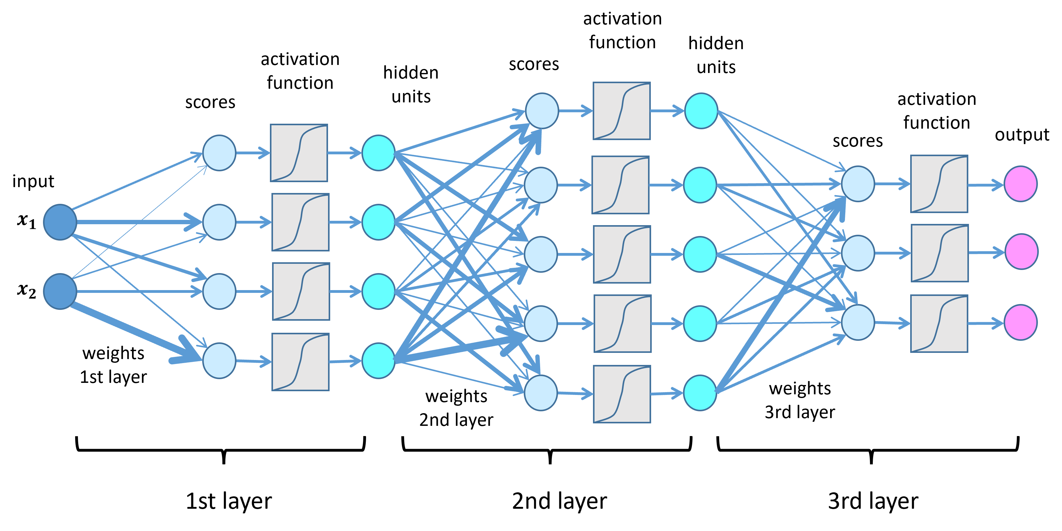
A neural network is a computational model inspired by biological brains. It consists of layers of interconnected “neurons” (mathematical functions) that transform input data into predictions.
Input → Hidden Layer 1 → Hidden Layer 2 → ... → Output
[Data]     [Transform]      [Transform]         [Prediction]
Key Components
- Neurons (Nodes)
Each neuron receives inputs, applies a weighted sum, adds a bias, and passes the result through an activation function:
\[y = \sigma(w_1x_1 + w_2x_2 + ... + w_nx_n + b)\]Where:
\(x_i\) are inputs
\(w_i\) are learned weights
\(b\) is a learned bias
\(\sigma\) is an activation function (ReLU, sigmoid, etc.)
- Layers
Neural networks are organized into layers that progressively transform input data. The input layer receives the raw features (geometry, topology), hidden layers perform transformations to extract meaningful patterns through learned weights and non-linear activations, and the output layer produces the final prediction (class probabilities for classification or continuous values for regression).
- Activation Functions
Activation functions introduce non-linearity into neural networks (meaning they can learn curves and complex patterns, not just straight lines), enabling them to learn complex patterns beyond simple linear relationships. The most commonly used activation is ReLU (Rectified Linear Unit), defined as \(f(x) = \max(0, x)\), which is both simple and effective. The sigmoid function \(f(x) = \frac{1}{1 + e^{-x}}\) outputs values between 0 and 1, making it suitable for binary probabilities. The tanh function \(f(x) = \tanh(x)\) outputs between -1 and 1, providing zero-centered activations. Finally, softmax converts raw scores (logits - the raw numbers output by the network before converting to probabilities) into a probability distribution over multiple classes for classification tasks.
Training Process
Training is the process of adjusting network weights to minimize errors:
Forward Pass: Input data flows through the network to produce predictions
Loss Calculation: Compare predictions to ground truth using a loss function
Backward Pass (also called backpropagation): Calculate gradients - mathematical measures of how much each weight contributed to the error - by working backwards through the network
Optimization: Update weights to reduce loss using an optimizer (an algorithm like Adam or SGD that decides how to adjust weights based on gradients)
This cycle repeats for many iterations (epochs) until the model converges.
Key Terminology:
Epoch: One complete pass through the entire training dataset
Batch: A subset of the dataset processed together (batch size = 32 means 32 samples at once)
Learning Rate: How big the weight update steps are (typical: 0.001 - 0.0001)
Overfitting: Model memorizes training data but fails on new data
Validation Set: Data held out during training to check for overfitting
Graph Neural Networks (GNNs)
Why GNNs for CAD Data?
CAD models have an inherent graph structure: faces connected by shared edges, edges meeting at vertices. Traditional neural networks (CNNs - Convolutional Neural Networks, fully-connected networks) expect fixed-size grid-like inputs (images, vectors), but CAD models have:
Variable topology: A simple box has 6 faces; a complex engine part may have thousands
Relational structure: Which faces are adjacent matters for understanding geometry (see CAD Fundamentals for Topology details)
Permutation invariance (order-independence): The order we list faces shouldn’t affect the result - face [A, B, C] should give the same answer as [C, A, B]
Graph Neural Networks are designed exactly for this type of structured, relational data.
Graph Representation of CAD Models
In HOOPS AI, a CAD B-rep model is represented as a graph where nodes correspond to CAD entities (faces, edges, or vertices depending on the task), and edges represent relationships between entities (such as face-adjacency or edge-face incidence). Each node carries node features - geometric properties like area, curvature, surface type, or sampled points - while edge features encode relationship properties such as shared edge length or dihedral angle between adjacent faces.
See also
For detailed examples of face-adjacency graphs and how CAD topology maps to graph structure, see CAD Fundamentals - “Face Adjacency Graph” section.

Boundary representation(BRep) and converting it to graph. The faces and curves in BRep correspond to the nodes and edges in graph.
How GNNs Work
GNNs operate through message passing (a process where each node collects and combines information from its neighboring nodes): each node aggregates information from its neighbors, updates its representation, and repeats for multiple layers.
Basic GNN Layer:
Note
Skip the equation? No problem! Think of it this way: each face learns about its neighbors, then their neighbors, and so on. After 3 layers, a face “knows” about faces up to 3 edges away.
Where:
\(h_i^{(l)}\) is the feature vector of node \(i\) at layer \(l\)
\(\mathcal{N}(i)\) are the neighbors of node \(i\)
\(\text{AGG}\) is an aggregation function (a way to combine multiple values into one, like taking the sum, mean, max, or attention-weighted average)
\(W^{(l)}\) are learnable weight matrices
\(\sigma\) is an activation function
Intuition: After \(L\) GNN layers, each node’s representation incorporates information from nodes up to \(L\) hops (steps through connections) away. For a 3-layer GNN on a face-adjacency graph, each face “knows about” the geometry of faces 3 edges away.
Tip
For Advanced Readers: The following research papers demonstrate these concepts in practice. You don’t need to read them to use HOOPS AI!
This message passing principle has been successfully applied across CAD ML research. BRepNet (Lambourne et al., 2021) introduced one of the first topological message passing systems specifically designed for B-rep models, using face-to-face and edge-to-face message passing to learn machining features. More recent work like GC-CAD (Quan et al., 2024) combines GNN message passing with UV-Net-style feature extraction and contrastive learning (a training technique that teaches the model to distinguish similar parts from dissimilar ones), achieving 100× speedup over classical shape descriptors while processing 360k CAD models.
Common GNN Architectures
- Graph Convolutional Network (GCN)
Simple and effective. Aggregates (combines) neighbor features using mean pooling (averaging all neighbor values together). BRepNet uses a variant of GCN for B-rep topology, where face nodes aggregate information from adjacent faces through shared edges.
# Conceptual (DGL handles the details)
new_features = activation(
    self_transform(node_features) +
    neighbor_transform(mean(neighbor_features))
)
- Graph Attention Network (GAT)
Graph Attention Networks use an attention mechanism (a learned weighting system that determines which inputs are most important) to weight neighbor contributions differently, learning which neighboring nodes are most important for each prediction. For example, when classifying a cylindrical hole feature, GAT might assign higher attention weights to adjacent planar faces than to distant curved surfaces. BrepMFR (2024) applies GAT with transformers for enhanced machining feature recognition, where the learned attention weights provide interpretability (the ability to understand why the model made a decision) - showing which adjacent faces the model considers most relevant when classifying each feature.
- Graph Transformer
Graph Transformers apply the transformer architecture (a modern neural network design originally created for language processing that uses attention to weigh the importance of different inputs) to graph-structured data, using attention mechanisms over all nodes rather than just immediate neighbors. This allows the model to capture long-range dependencies (relationships between distant parts of the model) across the entire part topology, though at higher computational cost. BRep-BERT (Lou et al., CIKM 2023) adapts BERT’s masked prediction approach (a training method where the model learns by trying to fill in deliberately hidden parts of the input) to B-rep graphs, pre-training (initial training on a large dataset before fine-tuning on a specific task) on Fusion 360 Gallery models through self-supervised learning (learning patterns from unlabeled data without human annotations) where the model learns to predict masked entities from context. This pre-training enables effective few-shot feature recognition (learning to recognize features from very few examples) even with limited labeled data.
- Message Passing Neural Networks (MPNN)
General framework where you can customize message, aggregation, and update functions.
Point Cloud Networks
Point cloud networks process 3D geometry as unordered sets of points, making them ideal for CAD surface sampling.
- PointNet
PointNet is the foundational architecture for point cloud processing (working with collections of 3D points in space), introducing a permutation-invariant design (meaning the output doesn’t change regardless of the order points are listed - [A,B,C] gives the same result as [C,A,B]) that can handle unordered sets of 3D points. The architecture processes each point individually through a shared Multi-Layer Perceptron (MLP), then aggregates (combines) all point features using max pooling (taking the maximum value across all points for each feature dimension) to produce a global feature vector. This max pooling operation is the key to permutation invariance - regardless of the order in which points are presented, the maximum value in each dimension remains constant. In CAD applications, PointNet processes UV grid samples (points sampled from the parametric surface representation of a face - see CAD Fundamentals for UV parameterization details) as unordered point clouds, where each point includes both position (x, y, z) and surface normal (a vector perpendicular to the surface indicating its orientation - see CAD Fundamentals) information (nx, ny, nz).
# Simplified PointNet flow
# Input: (N, 6) - N points with [x, y, z, nx, ny, nz]
point_features = shared_mlp(points)      # (N, 64)
global_feature = max_pool(point_features) # (64,) - single vector for entire face
classification = classifier(global_feature)
Mathematical Formulation:
\[f(\{x_1, ..., x_n\}) = \gamma \circ \text{MAX}_{i=1,...,n} \{\phi(x_i)\}\]Note
Math intimidating? Just remember: PointNet processes each point separately, then takes the maximum value across all points. HOOPS AI handles the implementation!
Where:
\(\phi\): Per-point feature extraction (shared MLP)
\(\text{MAX}\): Max pooling (symmetric aggregation)
\(\gamma\): Classification network
- PointNet++
PointNet++ extends the original PointNet with hierarchical processing to capture local geometric structures. The architecture uses multi-scale grouping of points through a series of set abstraction layers, where each layer samples a subset of points, groups nearby neighbors, and applies PointNet to extract local features. This hierarchical approach allows the network to capture fine geometric details that the original PointNet’s global pooling would miss, making it particularly effective for tasks requiring local context like segmentation and feature detection.
# Hierarchical processing
# Level 1: Sample 512 points, group neighbors, extract local features
centroids_1, features_1 = set_abstraction(points, num_points=512, radius=0.2)

# Level 2: Sample 128 points, group at larger radius
centroids_2, features_2 = set_abstraction(centroids_1, num_points=128, radius=0.4)

# Global feature
global_feature = max_pool(features_2)
Use Cases in CAD:
While pure point cloud methods are common for mesh data, UV-Net (Jayaraman et al., CVPR 2021) showed that structured UV parameterization (a mapping from 2D parameter space (u,v) to 3D surface coordinates - see CAD Fundamentals for details) with 2D CNNs outperforms unordered point clouds for B-rep CAD data. The paper demonstrated that sampling a regular 10×10 UV grid per face captures small features more reliably than random point sampling, as UV grids preserve spatial relationships. However, PointNet-style architectures remain useful for:
UV Grid Sampling: Flatten UV grids into point clouds with normals when spatial structure is less critical
Surface Characterization: Extract geometric features from face samples in a permutation-invariant manner
Multi-Face Aggregation: Process multiple faces independently, then combine using max pooling or attention
Hybrid Approaches: Self-Supervised Representation Learning for CAD (Jones et al., CVPR 2023) combines UV parametric sampling with implicit SDF reconstruction (learning a continuous function that represents distance to the surface - SDF stands for Signed Distance Field), using point cloud techniques to approximate per-face signed distance fields from UV-sampled points.
Tip
Advanced Research Note: The papers referenced above are for readers interested in the academic background. You don’t need to understand these to use HOOPS AI’s point cloud and UV grid features!
Convolutional Neural Networks (CNNs)
CNNs process grid-structured data (images, UV grids) using learnable filters. The breakthrough application of CNNs to CAD came with UV-Net (Jayaraman et al., CVPR 2021, GitHub), which demonstrated that 2D convolutions on UV parametric grids (2D grids of sampled points from CAD surface parameterization - see CAD Fundamentals) could effectively learn B-rep geometry while preserving topological structure through face adjacency graphs.
Key Concepts:
CNNs operate through convolution - sliding learnable filters over the input to detect local patterns like edges and textures. Pooling operations downsample the spatial dimensions (reduce the grid size), reducing computational cost while adding translation invariance (the network recognizes patterns regardless of their position in the grid). The architecture learns hierarchical features: early convolutional layers detect simple patterns (edges, corners), while deeper layers combine these to recognize complex shapes and geometric structures.
See also
New to CNNs? See Tutorials for hands-on examples, or check the glossary for quick definitions!
2D CNN for UV Grids:
import torch.nn as nn

class UVGridCNN(nn.Module):
    def __init__(self):
        super().__init__()
        # Input: (batch, 6, height, width) - 6 channels: x,y,z,nx,ny,nz
        self.conv1 = nn.Conv2d(6, 32, kernel_size=3, padding=1)
        self.conv2 = nn.Conv2d(32, 64, kernel_size=3, padding=1)
        self.pool = nn.MaxPool2d(2, 2)
        self.fc = nn.Linear(64 * 8 * 8, 128)  # Assuming 32x32 input -> 8x8 after pooling

    def forward(self, uv_grid):
        x = torch.relu(self.conv1(uv_grid))
        x = self.pool(x)
        x = torch.relu(self.conv2(x))
        x = self.pool(x)
        x = x.view(x.size(0), -1)  # Flatten
        features = self.fc(x)
        return features
Why CNNs for UV Grids?
The effectiveness of CNNs on UV grids was rigorously demonstrated in UV-Net (Jayaraman et al., CVPR 2021), which showed that 2D convolutions outperform point cloud methods (PointNet) on the SolidLetters classification benchmark. The key insight is that nearby points in UV parameter space correspond to nearby points on the physical surface, enabling CNNs to learn local geometric patterns just as they detect edges in images. Convolutional filters naturally detect curvature changes, ridges, and holes, producing consistent fixed-size feature vectors regardless of grid resolution (whether 10×10 or 32×32). The architecture handles UV seam discontinuities on cylindrical and toroidal surfaces through periodic padding (discussed in the supplementary material), and pooling layers capture patterns at multiple scales - from fine details like small fillets to global shape characteristics like overall surface curvature. Subsequent work like Self-Supervised Representation Learning for CAD (Jones et al., CVPR 2023) extended this approach by combining UV-grid CNNs with implicit SDF reconstruction (SDF = Signed Distance Field - a continuous function representing distance to the surface), pre-training on 1M unlabeled ABC models to achieve state-of-the-art few-shot learning.
Tip
For Advanced Readers: The research papers above provide academic context for HOOPS AI’s CNN implementation, but you can use the UV grid features without reading them!
Hybrid Architectures for CAD
HOOPS AI supports hybrid architectures that combine multiple neural network types. These architectures are accessed through the FlowModel interface with specific architecture names. Modern CAD ML research has shown that combining different network types leverages complementary strengths: CNNs capture local geometry, GNNs model topology, and transformers (attention-based networks that can process sequential data and learn relationships between distant elements) handle long-range dependencies.
See also
Not familiar with these architectures? See Graph Neural Network (GNN) and Convolutional Neural Network (CNN) in the glossary, or review CAD Fundamentals for CAD-specific concepts!
UV-Net: Hybrid CNN-GNN Architecture (cnn_gnn)
The pioneering hybrid architecture from Autodesk Research (Jayaraman et al., CVPR 2021, GitHub) combines image processing with graph reasoning for comprehensive CAD understanding. Tested on five datasets including SolidLetters, Fusion 360 Gallery, and ModelNet, UV-Net demonstrated superior classification and segmentation compared to point cloud and voxel methods.
Architecture:
UV-Net’s architecture consists of three main components working in parallel and then fusing their outputs. The CNN component uses 2D convolutional layers to process UV grids (sampled face geometry), extracting local geometric features such as curvature patterns and surface characteristics. Simultaneously, the GNN component applies graph convolutional layers to the face-adjacency graph, capturing topological relationships between faces and propagating information across the model structure. These two feature streams are then combined in a fusion layer that concatenates the geometric features from the CNN with the topological context from the GNN. Finally, a classifier processes these combined features to produce the final prediction, leveraging both local geometric details and global structural understanding.
When to Use:
UV-Net is most effective for tasks requiring both local geometric understanding and global topological context, such as face-level classification (e.g., surface type prediction) or part segmentation. It works best with datasets where UV parameterization is available for all faces.
HOOPS AI Implementation:
UV-Net is implemented in HOOPS AI as the GraphClassification FlowModel, which wraps the Classification model (the UV-Net architecture implementation). The model uses the exact hybrid CNN-GNN architecture described in the UV-Net paper.
from hoops_ai.ml.EXPERIMENTAL import GraphClassification

# UV-Net architecture for part classification
model = GraphClassification(
    num_classes=10  # Number of part categories
)
See Parts Classification Model for complete GraphClassification usage examples and Tutorials for classification workflows.
BrepMFR: Transformer-based GNN Architecture with Domain Adaptation (transformer_gnn)
Advanced architecture using transformer attention (mechanism that allows models to focus on relevant parts of the input) for machining feature recognition with transfer learning (applying knowledge learned from one dataset to improve performance on another).
Architecture:
Graph Transformer: Applies transformer attention mechanism over graph nodes (faces)
Geometric Encoding: Encodes local geometric shapes using learned embeddings
Topological Encoding: Captures global relationships through multi-head attention
Domain Adaptation: Two-step training strategy to transfer from synthetic to real CAD data
Domain Adaptation Strategy:
Pre-training: Train on large synthetic CAD dataset
Fine-tuning: Adapt to real CAD data with domain adaptation loss
Transfer: Leverages synthetic data to overcome limited real-world labels
When to Use:
Machining feature recognition tasks
Limited real-world labeled data (use synthetic pre-training)
Tasks requiring long-range dependencies (transformer attention sees entire model)
HOOPS AI Implementation:
BrepMFR is implemented in HOOPS AI as the GraphNodeClassification FlowModel, which wraps the BrepSeg model (the BrepMFR architecture implementation). The model class is called BrepSeg but it implements the BrepMFR paper’s transformer-based graph neural network with domain adaptation capabilities.
from hoops_ai.ml.EXPERIMENTAL import GraphNodeClassification

# BrepMFR architecture for machining feature recognition
model = GraphNodeClassification(
    num_classes=24,        # 24 machining feature types
    n_layers_encode=8,     # Transformer layers
    dim_node=256,          # Node embedding dimension
    d_model=512,           # Model dimension
    n_heads=32,            # Attention heads
    dropout=0.3,
    attention_dropout=0.3
)
See Develop Your own ML Model for complete GraphNodeClassification usage examples and /tutorials/feature-recognition for machining feature recognition workflows.
PyTorch and PyTorch Lightning
HOOPS AI uses PyTorch as its deep learning framework, with PyTorch Lightning for training orchestration. PyTorch is an open-source machine learning library widely used in research and production, while Lightning provides a structured framework that simplifies training workflows.
See also
New to PyTorch? Check the official PyTorch tutorials for hands-on introduction, or see Tutorials for HOOPS AI-specific examples!
PyTorch Basics
- Tensors
Multi-dimensional arrays (similar to NumPy) that can run on GPUs (Graphics Processing Units - hardware accelerators for parallel computation):
import torch

# Create tensors
features = torch.tensor([[1.0, 2.0], [3.0, 4.0]])  # 2D tensor
labels = torch.tensor([0, 1])  # 1D tensor

# Move to GPU
features_gpu = features.cuda()
- Modules (Models)
Neural networks are defined as classes inheriting from
torch.nn.Module:import torch.nn as nn class SimpleClassifier(nn.Module): def __init__(self, input_dim, num_classes): super().__init__() self.fc1 = nn.Linear(input_dim, 128) self.fc2 = nn.Linear(128, num_classes) def forward(self, x): x = torch.relu(self.fc1(x)) x = self.fc2(x) return x
- Optimizers
Algorithms that update model weights during training using computed gradients (the direction and magnitude to adjust each weight):
Adam (Adaptive Moment Estimation): Automatically adjusts learning rates for each parameter, works well in most cases (HOOPS AI default)
SGD (Stochastic Gradient Descent): Updates weights using random batches of data, simpler but requires careful tuning of learning rate
PyTorch Lightning
PyTorch Lightning is a high-level wrapper that removes boilerplate code (repetitive setup) and adds best practices automatically.
Why Lightning?
Handles GPU/CPU switching automatically
Manages training/validation loops (no need to write
for epoch in range(num_epochs)yourself)Integrates logging and checkpointing (saves model progress during training)
Scales to multi-GPU training easily
LightningModule Structure:
import pytorch_lightning as pl

class MyModel(pl.LightningModule):
    def __init__(self):
        super().__init__()
        self.model = build_network()

    def forward(self, x):
        """Forward pass - how data flows through the model"""
        return self.model(x)

    def training_step(self, batch, batch_idx):
        """What happens for each training batch"""
        x, y = batch
        predictions = self(x)
        loss = compute_loss(predictions, y)
        self.log('train_loss', loss)
        return loss

    def validation_step(self, batch, batch_idx):
        """What happens for each validation batch"""
        x, y = batch
        predictions = self(x)
        accuracy = compute_accuracy(predictions, y)
        self.log('val_accuracy', accuracy)

    def configure_optimizers(self):
        """Define optimizer and learning rate schedule"""
        return torch.optim.Adam(self.parameters(), lr=0.001)
Trainer:
The Trainer handles the entire training loop:
from pytorch_lightning import Trainer

trainer = Trainer(
    max_epochs=100,           # Train for 100 epochs
    accelerator='gpu',        # Use GPU if available
    devices=1,                # Use 1 GPU
    log_every_n_steps=10,    # Log metrics every 10 batches
)

trainer.fit(model, train_dataloader, val_dataloader)
DGL: Deep Graph Library
HOOPS AI uses DGL (Deep Graph Library) for efficient graph neural network operations. DGL is an open-source Python library optimized for GNN training on both CPUs and GPUs.
See also
New to graph libraries? See the DGL tutorials for hands-on introduction, or start with Tutorials for HOOPS AI-specific examples!
DGL Graph Structure
import dgl
import torch

# Create graph from edge list
# Face-adjacency: face 0 connects to faces 1,2,3
src = [0, 0, 0, 1, 1, 2]
dst = [1, 2, 3, 2, 3, 3]
graph = dgl.graph((src, dst))

# Add node features (face geometric properties)
graph.ndata['features'] = torch.randn(4, 64)  # 4 faces, 64-dim features

# Add edge features (relationship properties)
graph.edata['edge_attr'] = torch.randn(6, 16)  # 6 edges, 16-dim features
Batching Multiple Graphs:
When training on multiple CAD models, DGL batches graphs into a single large graph (combines multiple small graphs into one big graph for efficient parallel processing):
# Batch 3 CAD models (graphs) together
graphs = [graph1, graph2, graph3]
batched = dgl.batch(graphs)  # Creates one large graph with disconnected components

# Process entire batch through GNN in parallel
output = gnn_model(batched, batched.ndata['features'])
PyTorch Geometric: Alternative Graph Library
While HOOPS AI primarily uses DGL, PyTorch Geometric (PyG) is another popular graph deep learning library. PyG provides similar functionality to DGL with a slightly different API design.
See also
Want to learn PyG? See the PyTorch Geometric documentation for comprehensive tutorials!
When You Might See PyTorch Geometric
PyTorch Geometric may appear in:
Research code: Many GNN papers provide PyG implementations
External tutorials: CAD ML tutorials often use PyG for examples
Custom implementations: Users extending HOOPS AI with custom architectures
PyG Graph Structure
import torch
from torch_geometric.data import Data

# Create graph from edge list
# Edge index: [source_nodes, destination_nodes]
edge_index = torch.tensor([[0, 0, 0, 1, 1, 2],  # Source nodes
                           [1, 2, 3, 2, 3, 3]], # Destination nodes
                          dtype=torch.long)

# Node features
x = torch.randn(4, 64)  # 4 faces, 64-dim features

# Edge features
edge_attr = torch.randn(6, 16)  # 6 edges, 16-dim features

# Create PyG Data object
graph = Data(x=x, edge_index=edge_index, edge_attr=edge_attr)
Converting Between DGL and PyTorch Geometric:
# DGL to PyG
def dgl_to_pyg(dgl_graph):
    edge_index = torch.stack(dgl_graph.edges())
    x = dgl_graph.ndata['features']
    edge_attr = dgl_graph.edata.get('edge_attr', None)
    return Data(x=x, edge_index=edge_index, edge_attr=edge_attr)

# PyG to DGL
def pyg_to_dgl(pyg_data):
    src, dst = pyg_data.edge_index
    g = dgl.graph((src, dst))
    g.ndata['features'] = pyg_data.x
    if pyg_data.edge_attr is not None:
        g.edata['edge_attr'] = pyg_data.edge_attr
    return g
Key Differences:
Aspect |
DGL |
PyTorch Geometric |
|---|---|---|
Graph Storage |
Graph object with ndata/edata |
Data object with x/edge_index |
Batching |
|
|
Message Passing |
Functional API ( |
Layer-based ( |
HOOPS AI Usage |
Primary library (recommended) |
Not directly used (but compatible) |
Why HOOPS AI Uses DGL:
Efficient batching: Better performance for variable-size CAD graphs (different models have different numbers of faces)
Flexible message passing: Easier to customize for CAD-specific operations (like handling B-rep topology)
Integration: Better integration with the existing HOOPS AI pipeline
Loss Functions
Loss functions measure how wrong the model’s predictions are. HOOPS AI uses different losses for different tasks.
Cross-Entropy Loss (Classification)
For predicting discrete classes (part type, feature type):
Where:
\(y_i\) is the true label (one-hot encoded, meaning a vector where only the correct class is 1 and all others are 0, like [0, 1, 0, 0] for class 2)
\(\hat{y}_i\) is the predicted probability distribution (after applying softmax, which converts raw scores to probabilities that sum to 1)
\(C\) is the number of classes
import torch.nn.functional as F

# Model outputs logits
logits = model(graph, features)  # Shape: [batch_size, num_classes]

# Compute loss
loss = F.cross_entropy(logits, labels)
Intuition: Penalizes confident wrong predictions more than uncertain ones (predicting 90% confidence for the wrong class is penalized more than 60% confidence).
Binary Cross-Entropy (Node Classification)
For binary classification on each node (e.g., is this face a hole?):
Where \(N\) is the number of nodes (faces), \(y_i\) is 0 or 1 (binary label), and \(\hat{y}_i\) is predicted probability.
Mean Squared Error (Regression)
For predicting continuous values (like surface area or curvature):
Where \(y_i\) is the true value and \(\hat{y}_i\) is the predicted value. MSE penalizes large errors quadratically (an error of 2 is penalized 4 times more than an error of 1).
Advanced Concepts
This section covers advanced ML techniques used in CAD research. These concepts are optional - you can build effective HOOPS AI models without them!
Important
Advanced Section! The following topics are for readers interested in cutting-edge research. You can skip to Tutorials to start building models immediately!
Transfer Learning and Domain Adaptation
Transfer Learning: Use a model pre-trained on one dataset (e.g., synthetic CAD) and fine-tune (continue training with a smaller learning rate) on another (e.g., real CAD).
# Load pre-trained weights (saved model parameters)
model = MyGNNModel.load_from_checkpoint("pretrained.ckpt")

# Fine-tune on new dataset with smaller learning rate
trainer = FlowTrainer(
    flowmodel=flow_model,
    dataset_loader=new_dataset,
    learning_rate=0.0001,  # 10x smaller for fine-tuning
    max_epochs=50
)
Domain Adaptation: Techniques to reduce the gap between training data (synthetic) and real-world data:
Adversarial training: Train the model to make features domain-invariant (features that look the same whether they come from synthetic or real data)
Data augmentation (creating variations of existing data): Add noise, rotations, variations to synthetic data to make the model more robust
Progressive fine-tuning: Train on synthetic → fine-tune on small real dataset
Tip
For Advanced Readers: Transfer learning and domain adaptation are research topics explored in papers like Self-Supervised Representation Learning for CAD (Jones et al., CVPR 2023). HOOPS AI supports these workflows through the FlowTrainer interface!
Regularization Techniques
Methods to prevent overfitting (when the model memorizes training data instead of learning general patterns):
- Dropout
Randomly “drop” (set to zero) neurons during training to prevent co-adaptation (where neurons become too dependent on each other):
self.dropout = nn.Dropout(p=0.5)  # Drop 50% of neurons randomly
x = self.dropout(x)
- Weight Decay
Add penalty for large weights (L2 regularization, meaning the sum of squared weights is added to the loss) to prevent overfitting:
optimizer = torch.optim.Adam(model.parameters(),
                             lr=0.001,
                             weight_decay=1e-5)  # Penalty coefficient
- Early Stopping
Stop training when validation performance stops improving (prevents wasting time and overfitting):
from pytorch_lightning.callbacks import EarlyStopping

early_stop = EarlyStopping(
    monitor='val_accuracy',
    patience=10,  # Stop if no improvement for 10 epochs
    mode='max'
)
trainer = Trainer(callbacks=[early_stop])
Attention Mechanisms
Attention allows models to focus on important parts of the input (e.g., which faces are most relevant for predicting a machining feature).
Where Q (query), K (key), and V (value) are learned transformations of the input. The softmax operation produces weights that determine how much to “attend to” each input element.
In CAD context:
Graph Attention: Learns which neighboring faces are most relevant (e.g., holes matter more than outer shells for certain features)
Transformer Attention: Captures long-range dependencies across the entire model (e.g., detecting symmetry patterns)
Self-Supervised Learning
Learning useful representations without manual labels (useful when labeled CAD data is expensive to obtain):
- Contrastive Learning
Learn to distinguish between similar and dissimilar samples:
Positive pairs: Different views of the same CAD model (e.g., different rotations or UV samplings)
Negative pairs: Different CAD models entirely
Goal: Make representations (the feature vectors produced by the encoder) of positive pairs similar, negative pairs different
- Masked Prediction (BERT-style)
Hide parts of the input and predict them (like filling in blanks):
Mask certain faces in a CAD model (hide their features)
Train the model to predict their properties from surrounding context
Used in BRep-BERT architecture (BERT stands for Bidirectional Encoder Representations from Transformers - a self-supervised learning approach)
Best Practices for CAD Machine Learning
This section provides practical guidelines for building effective CAD ML models with HOOPS AI.
See also
For hands-on examples demonstrating these practices, see Tutorials!
Data Quality
Balanced datasets: Ensure each class has sufficient examples (aim for 100+ per class to avoid class imbalance, where the model ignores rare classes)
Clean labels: Verify ground truth labels are accurate (incorrect labels = model learns wrong patterns)
Representative data: Include variation (simple/complex parts, different manufacturers) to ensure generalization (ability to work on unseen data)
Consistent preprocessing: Use the same encoding settings for train/test data (e.g., same UV grid resolution)
Feature Engineering
Normalization (scaling features to similar ranges, typically [0,1] or mean=0 std=1): Scale features to prevent some from dominating others
# Area in [0.01, 1000] m² → normalize to [0, 1] using min-max scaling
normalized_area = (area - area_min) / (area_max - area_min)
Domain knowledge: Include CAD-specific features (surface type, curvature, convexity - see CAD Fundamentals for CAD concepts)
Multi-scale features: Combine local (face-level) and global (model-level) information for richer representations
Model Training
Start simple: Try a basic GCN before complex architectures (simpler models are easier to debug and may work just as well)
Monitor overfitting: Track train vs. validation metrics (if train keeps improving but validation plateaus or worsens, you’re overfitting)
Use checkpoints: Save best model based on validation performance (not final epoch!)
Visualize training: Use TensorBoard to spot issues early (loss spikes, overfitting trends)
Ablation studies (systematically removing features/components to see what’s actually needed): Test which features matter most for your task
Debugging ML Models
Common Issues:
Loss not decreasing:
Check learning rate (try 1e-3, 1e-4, 1e-5)
Verify data preprocessing (normalized? correct shapes?)
Inspect first batch manually (print values, check for NaN or extreme outliers)
Overfitting (train accuracy high, validation low):
Add dropout (start with p=0.3)
Reduce model complexity (fewer layers, smaller hidden dimensions)
Get more training data (or use data augmentation)
Use regularization (weight decay, early stopping)
Underfitting (both train and validation accuracy low):
Increase model capacity (more layers, wider layers - increase hidden_dim)
Train longer (more epochs)
Add more relevant features (see CAD Data Encoding for feature extraction options)
Unstable training (loss oscillates or explodes):
Reduce learning rate (divide by 10)
Use gradient clipping (limiting gradient magnitudes to prevent extreme updates)
Check for data issues (NaN values, extreme outliers, incorrect normalization)
Resources and Further Reading
For Beginners:
Tutorials: Hands-on HOOPS AI introduction
CAD Fundamentals: CAD concepts for ML practitioners
Glossary: Quick reference for ML and CAD terms
Concepts:
Graph Neural Networks: Geometric Deep Learning Grids, Groups, Graphs, Geodesics, and Gauges
PyTorch: Official PyTorch Tutorials
PyTorch Lightning: Lightning Documentation
DGL: DGL User Guide
CAD ML Research:
Next Steps
Read CAD Fundamentals to understand B-rep representation
Follow Tutorials for hands-on examples
Explore API Reference for detailed class documentation
Additional Resources:
Glossary for quick term definitions
CAD Data Encoding for practical feature extraction examples
Tutorials for step-by-step walkthroughs