Defining a Scene Graph
Overview
This section provides guidelines on how to design scene graphs for a variety of application types, and assumes familiarity with the database concepts located in the Programming Guide, here. Most importantly, when creating your scene graph and setting model-specific attributes, you should be aware of the performance information reviewed in the segment performance section and the geometry section of the guide.
All of the guides depict a scene graph that is created underneath a main ‘model’ segment, which would then be included by one or more ‘views’. If you are using HOOPS/MVO, this starting segment hierarchy is implicitly created when instantiating the HOOPS/MVO HBaseModel and HBaseView objects, and you would create the model underneath the preexisting ‘model’ segment. If you are not using HOOPS/MVO, you will need to manually create this view/model segment hierarchy.
HOOPS/MVO also has built-in support for exporting/importing the model data to/from several file formats. However, you may not be using MVO, or may need to write your own custom logic for model export/import. In either case, you should export the scene graph starting with the contents of the ‘model’ segment, and likewise import a scene graph into the ‘model’ segment.
This document makes several references to files from the ‘datasets’ package. This package is available as a separate download from the Tech Soft 3D Developer Zone.
Scene Graph Examples
AEC/GIS/ECAD
This describes the scene graph that would typically be created by applications in the AEC, ECAD, and GIS markets. These application types commonly deal with 2D information distributed among various layers, which need to be independently manipulated, ordered, and styled.
Organizing the Scene Graph
These types of applications primarily contain 2D geometry that exists in a single plane. When inserting such geometry into the HOOPS Visualize database, the z-values of the insertion points should be zero. HOOPS Visualize will detect this and automatically make some internal optimizations.
Since the geometry representing the model resides in the same plane, it must be distributed among different layers. The layers may need to be independently:
- drawn with a specific order relative to other layers
- highlighted
- hidden
- modified (their position may need to change, or they may need to be drawn with different attributes such as color, line style, line thickness, etc…)
- deleted
Organizing the HOOPS Visualize scene graph to represent layers is quite easy. Underneath the main ‘model’ segment, we create a sibling segment for each layer in the model. Each layer segment would in turn contain geometry and any additional subsegment tree that represents that layer. All of the aforementioned functionality can easily be achieved by modifying the appropriate attributes in the top level segment for each layer. The following diagram shows how the scene graph might look:
Reusing Objects
The scene graph in the previous section implies that a layer’s geometry is directly stored in the layer segment (or subsegment tree). This may be valid for some applications, but it is common for the model to contain ‘template’ objects that need to be referenced multiple times (perhaps by a single layer, or maybe by many layers). The more efficient way to represent this scenario is to store the template objects inside of separate segments, and then reference those objects into the main model hierarchy by using Include_Segment as necessary:
When creating the model using HOOPS/MVO, the ‘Model’ segment already exists and the HOOPS/3dGS pseudo-code corresponding with the blue portions of the diagram is listed below. Notice that we set Visibility to ‘off’ at the top of the object library, since we don’t want the contents of those segments to be automatically visible when the scene is drawn. We only want them to be visible as a result of being included into the model’s ‘layer’ segments:
// define the model
HC_Open_Segment("?Include Library");
        HC_Open_Segment("Model_0");

                HC_Open_Segment("Object Library");
                        HC_Set_Visibility("off");

                        HC_Open_Segment("Object_1");
                                // define an object here
                        HC_Close_Segment();

                        HC_Open_Segment("Object_2");
                                // define an object here
                        HC_Close_Segment();

                HC_Close_Segment();


                HC_Open_Segment("Layer_1");
                        // define the layer
                HC_Close_Segment();

                HC_Open_Segment("Layer_2");
                        HC_Include_Segment("../Object Library/Object_1");
                        // define the remainder of the layer
                HC_Close_Segment();

                HC_Open_Segment("Layer_3");
                        HC_Include_Segment("../Object Library/Object_2");
                        // define the remainder of the layer
                HC_Close_Segment();
        HC_Close_Segment();   // close "Model_0"
HC_Close_Segment();     // close "?Include Library"

// include the model into the scene
HC_Open_Segment("?driver/opengl/window0");
        HC_Open_Segment("Scene");
                HC_Include_Segment("?Include Library/Model_0");
        HC_Close_Segment();
HC_Close_Segment();
Ordering Layers
Ordering layers in a 2D scene is frequently necessary, as they may need a specific drawing order. (This would be similar to bringing 2D objects to the front or sending them to the back in an application like Visio or Word.) HOOPS/3dGS segments can be manually reordered with respect to one another using a variety of techniques, discussed in this section of the HOOPS/3dGS Programming Guide.
MCAD/3D
This describes the scene graph that would typically be created by Mechanical CAD, 3D Viewing or ‘generic’ 3D applications. It discusses how to represent assembly, part, body, and edge topology, and also reviews efficient segment organization for 3D data.
Organizing the Data for MCAD
The main concept that dominates scene graph organization for 3D and Mechanical CAD applications is to use segments/segment-trees to represent parts of the 3D model that are logically grouped together. The HOOPS/3dGS segment-hierarchy should generally mimic the assembly/part hierarchy for an MCAD application, or the part hierarchy for an application that works with kinematics on 3D models. (We should stress the word ‘generally’ because the scene graph should also be optimized for graphics drawing, which may cause it to diverge somewhat from the application’s assembly/kinematics hierarchy.)
Grouping logical parts of the 3D model into individuals segments facilitates modification of their attributes, such as visibility, color or modelling matrix. For example, if a part will need to be independently moved, it must either reside in it’s own unique segment (since each segment has a modelling matrix which affects everything in the segment), or the geometry representing the part would need to be moved into a new segment. Being able to simply change the modelling matrix on the existing segment is easier to manage.
MCAD
MCAD applications usually have an assembly structure and corresponding topology structure. The highest level representation is typically an assembly, which contain parts, each of which contain bodies. Bodies, in turn, can contain the topological concepts of faces (a sub region of a body) and edges.
- A segment is used to represent each assembly, part and body. The assembly parts/bodies may reference objects from a master ‘object_library’ to reuse them, and/or the parts/bodies may be defined in place underneath the assembly/part hierarchy.
- A single shell is used to represent a body. Shells can be independently styled (visibility, color, etc…) Sometimes, applications also need to set attributes on the topological ‘faces’. While it may be tempting to use a shell for each ‘face’ in order to more easily achieve this, the HOOPS/3dGS shell primitive supports attributes on subparts, and also supports a concept of regions (where you would define a region for each ‘face’). Therefore, using a single shell per body will permit the desired functionality in the majority of situations, and is the preferred approach since it is more optimal from a memory, performance and HSF data compression standpoint. Thoroughly read the section on shells and the geometry performance section of the HOOPS/3dGS Programming Guide for information on proper shell usage and optimization.
- Lines/polylines/circles/arcs are used to represent the edges of a body, and are inserted in the ‘body’ segment. (Note: when representing wire circles, it is best to use an elliptical arc. This is discussed in more detail in circles and ellipses section).
The following scene graph provides an example:
The HOOPS/3dGS pseudo-code corresponding with the blue portions of the diagram is listed below. Notice that we set Visibility to ‘off’ at the top of the object library, since we don’t want the contents of those segments to be automatically visible when the scene is drawn. We only want them to be visible as a result of being included into the model’s ‘assembly’ segments:
// define the model

HC_Open_Segment("?Include Library");

  HC_Open_Segment("Model_0");

        HC_Open_Segment("Object Library");
          HC_Set_Visibility("off");

          HC_Open_Segment("Object_1");
                // insert geometry defining this reusable object
                // set any attributes that are a fixed property of the object
          HC_Close_Segment();

        HC_Close_Segment();


        HC_Open_Segment("Assembly");

          HC_Open_Segment("Part_1");
                HC_Open_Segment("Body_1");
                  // define the body using shells, lines, arcs, etc...
                HC_Close_Segment();
                HC_Open_Segment("Body_2");
                  // define the body using shells, lines, arcs, etc...
                HC_Close_Segment();
          HC_Close_Segment();

          HC_Open_Segment("Part_2");
                HC_Open_Segment("Body_1");
                  HC_Include_Segment("../../../Object Library/Object_1");
                  // define the remainder of the body in place, by using shells, lines, arcs, etc...
                HC_Close_Segment();

                HC_Open_Segment("Body_2");
                  HC_Include_Segment("../../../Object Library/Object_1");
                  // define the remainder of the body in place, by using shells, lines, arcs, etc...
                HC_Close_Segment();
          HC_Close_Segment();

        HC_Close_Segment();  // close "Assembly"

  HC_Close_Segment();    // close "Model_0"

HC_Close_Segment();      // close "?Include Library"


// include the model into the scene

HC_Open_Segment("?driver/opengl/window0");
  HC_Open_Segment("Scene");
        HC_Include_Segment("?Include Library/Model_0");
  HC_Close_Segment();
HC_Close_Segment();
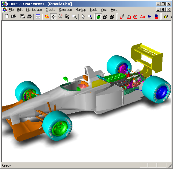
Let’s explore the scene graph of a real assembly. Run the HOOPS Part Viewer and load in /datasets/hsf/cad/formula1.hsf from the datasets package. Visually explore its scene graph in a dynamic fashion by opening the ‘Segment Browser’ dialog. Additionally, review the ASCII readable version of formula1.hsf (and thus the scene graph), by saving the HSF file out to an HMF file and then loading it into a text editor.
General 3D Models
There is not a set of hard and fast rules for organizing the scene graph when you have arbitrary 3D data. Rather, you should focus on keeping segments to a minimum (i.e. creating new segments when they are actually necessary), and making your shells as large as possible.
Let’s take the simple example of the solar system. We’ll need to design a segment tree which can enables us to accurately simulate how planets and their moons move about the system over time. Because each object has local behaviors (such as a rotation, etc..), it needs to have it’s own local object space, and therefore needs a segment associated with it. The segment containing each solar system object will include a template object called ‘celestial object’, which contains a shell denoting a sphere. Then, each segment in the solar system hierarchy will apply a scaling factor depending on the size of the object, along with any other attributes specific to that object.
If we want to model the sun, the earth and moon for starters, we would need the segment tree in the following diagram:
The HOOPS/3dGS pseudo-code corresponding with the blue portions of the diagram is listed below:
// define the model

HC_Open_Segment("?Include Library");

  HC_Open_Segment("Model_0");

        HC_Open_Segment("Object Library");
          HC_Set_Visibility("off");

          HC_Open_Segment("Celestial Object");
                // define the object
                HC_Insert_Shell(...);

                // set attributes that are a fixed property of the master object
                HC_Set_Color(...);
          HC_Close_Segment();

        HC_Close_Segment();


        HC_Open_Segment("Solar System");

          HC_Open_Segment("Earth");
                HC_Open_Segment("Planet");
                  HC_Include_Segment("../../../Object Library/Celestial Object");
                  HC_Scale_Object(...);
                HC_Close_Segment();
                HC_Open_Segment("Moon");
                  HC_Include_Segment("../../../Object Library/Celestial Object");
                  HC_Scale_Object(...);
                HC_Close_Segment();
          HC_Close_Segment();

          HC_Open_Segment("Sun");
                HC_Include_Segment("../../../Object Library/Celestial Object");
                HC_Scale_Object(...);
          HC_Close_Segment();


        HC_Close_Segment();  // close "Solar System"

  HC_Close_Segment();    // close "Model_0"

HC_Close_Segment();      // close "?Include Library"


// include the model into the scene

HC_Open_Segment("?driver/opengl/window0");

  HC_Open_Segment("Scene");
        HC_Include_Segment("?Include Library/Model_0");
  HC_Close_Segment();

HC_Close_Segment();
The ‘planet’, ‘moon’, and ‘sun’ segments would also contain several other rotation and translation operations if we wanted to accurately position and animate them. Refer to the Programming Guide on :doc:modelling matrices </prog_guide/3dgs/03_3_viewing_modelling_matrices>` for more information on how modelling matrices would be applied to accurately model and animate the solar system example.
Hybrid 2D/3D
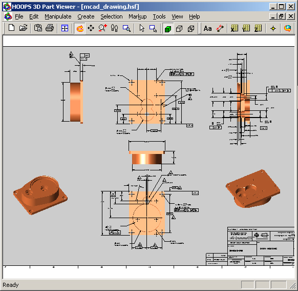
This describes a scene graph whose 3D model is based on the 3D/MCAD scene graph discussed above, but incorporates concepts required by ‘design intent’ applications in the CAD market. These are applications that contain 3D part data, but also overlay 2D annotation data on the 3D objects, and layout multiple views of the model in preparation for hardcopy.
Organizing the Data in Hybrid Scenes
Many design-intent and MCAD applications need to display several views of a 3D model, with each view having a unique orientation and set of view-specific 2D annotations. These views may exist as part of an overall drawing that contains it’s own annotation information, background color, etc. Since there are both 2D and 3D aspects to the scene graph, you should review the AEC/GID/ECAD and 3D/MCAD scene graph documents.
Such a hybrid scene graph typically includes the following concepts:
3D model library
This is the repository for the master model, which should generally be designed with the 3D/MCAD scene graph principles in mind. The HOOPS/3dGS ‘shell’ primitive would be used to represent your 3D objects. Each part would ideally have a segment, which in turn would have a single segment for each body. This segment would have it’s visibility turned off, since we’d only want parts to show up in the main drawing if they were specifically included by the views.
Drawing
- This is the segment that corresponds with the top of the ‘viewable’ scene graph. It contains a subsegment for each ‘view’ of the model, as well as a separate segment for the ‘border’ of the drawing.
- The ‘border’ has a ‘paper’ subsegment containing the geometry for the drawing background (a polygon, typically). This paper segment has a “depth range” setting that pushes it to the background. Refer to this subsection of the Programming Guide for more information about ordering geometry.
Views
- Each view contains a translation that places it at the correct location on the virtual drawing, and contains two subsegments: one for the the ‘model’, and another for ‘markup’ information.
- The ‘markup’ subsegment contains the 2D annotation information.
- The ‘model’ subsegment includes parts from the 3D model library as necessary, and applies transforms specific to the view. It could contain a polygonal clip region setting (
Set_Polygonal_Clip_Region), which has the effect of defining another software viewport within the scene. Anything outside the region (that’s in the containing segment or subsegments) gets clipped.
The diagram below depicts how the scene graph might look:
The HOOPS/3dGS pseudo-code corresponding with the blue portions of the diagram is listed down below. This code actually corresponds with the scene graph contained in the /datasets/hsf/cad/mcad_drawing.hsf file located in the datasets package (a screenshot of this HSF file is included at the beginning of this document). Visually explore its scene graph in a dynamic fashion by loading it into the HOOPS 3D Part Viewer, and then opening the ‘Segment Browser’ dialog. Additionally, review the ASCII readable version of mcad_drawing.hsf (and thus the scene graph), by saving the HSF file out to an HMF file and then loading it into a text editor:
// define the model

HC_Open_Segment("?Include Library");

  HC_Open_Segment("Model_0");

        HC_Open_Segment("drawing");

          HC_Open_Segment("view1");

                HC_Set_Modelling_Matrix(...);   // translate the view

                HC_Open_Segment("model");
                  // define the model using shells
                  // turn off the visibility of 'edges' (to hide the implicit 'shell' edges)
                  HC_Set_Modelling_Matrix(...);   // rotate the view
                HC_Close_Segment();

                HC_Open_Segment("markup");
                  // insert geometry to represent the 2D annotations
                HC_Close_Segment();

          HC_Close_Segment();  // close "view1"


          HC_Open_Segment("border");

                // insert geometry representing the border annotations (text, polylines, polygons, etc...)

                HC_Open_Segment("paper");
                  HC_Set_Rendering_Options("depth range = (1,1)");
                HC_Close_Segment();

          HC_Close_Segment();  // close "border"

        HC_Close_Segment();    // close "drawing"


        HC_Open_Segment("library");
          HC_Set_Visibililty("off");

          HC_Open_Segment("master_objects");
                HC_Open_Segment("object1");
                  // insert geometry defining this reusable object
                  // set any attributes that are a fixed property of the object
                HC_Close_Segment();
          HC_Close_Segment();

          HC_Open_Segment("part");
                HC_Open_Segment("body1");
                  // define the body using shells, lines, arc, etc...
                  HC_Include_Segment(../../master_objects/object1");
                HC_Close_Segment();
          HC_Close_Segment();

        HC_Close_Segment();  // close "library"

  HC_Close_Segment();    // close "Model_0"

HC_Close_Segment();      // close "?Include Library"


// include the model into the scene

HC_Open_Segment("?driver/opengl/window0");
  HC_Open_Segment("Scene");
        HC_Include_Segment("?Include Library/Model_0");
  HC_Close_Segment();
HC_Close_Segment();
Computer-Aided Engineering
This describes the scene graph common to Computer Aided Engineering applications which include Finite Element Analysis (FEA) and virtual prototyping/simulation applications. It reviews concepts such as creating legend bars, applying color contour info to the model, and using the various face/edge visibility capabilties available in HOOPS/3dGS. This document focuses on the post-processor aspects of these applications. You should refer to the 3D/MCAD document above if you’re designing a scene graph for a pre-processor.
Organizing the Data in CAE Scenes
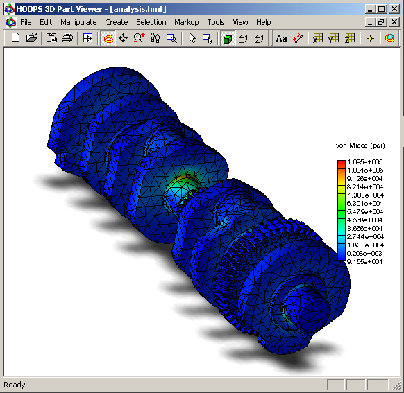
The post-processor component of a Finite Element Analysis application, along with many virtual prototyping/simulation applications, typically displays a 3D model that has color data mapped to it. This color data represents the ‘solved’ model (The original CAD model gets sent to a mesher, and then the ‘mesh’ version is ‘solved’ for one or more variables, such as heat, stress, fluid flow, electromagnetic field, deformation, etc…) A legend bar is also commonly displayed so the end-user can see the relationship between color and results. Here are some general guidelines to follow when organizing the scene graph:
3D Model
- The model should generally be designed with the 3D/MCAD scene graph principles in mind. The HOOPS/3dGS ‘shell’ primitive would be used to represent your 3D objects (meshes).
- When representing the edges/wires of your model/mesh, the implicit edges of the HOOPS ‘shell’ primitive may not be adequate for display purposes, since they are simply the edges bordering the ‘faces’ that defined the point connectivity. For example, the triangles in your mesh may need to be ‘internally’ tesselated into 4 triangles to get the correct color interpolation. If you simply turned on the shell edges in this case, you would see a lot more edges in the scene (you’d see three additional edges on each shell face), but perhaps the only edges you wish to see are those bordering the ‘original’ pre-tesselation triangles. In this case, you could turn off edge visibility, and insert dedicated polylines to represent the edges of interest.
- The color data is mapped by calling ::Set_Rendering_Options and setting the ‘color interpolation’ and ‘color index interpolation’ options. Refer to that section of the HOOPS/3dGS Programming Guide for more detailed usage information.
Legend Bar
- A separate top-level segment in the ‘model’ will store the scene graph components that represent the legend bar.
- The
Compute_Circumcuboidfunction is used to calculate scene extents, and then the camera is reset appropriately. (If you’re using HOOPS/MVO, theHBaseView::FitWorldroutine does this work for you.) However, we want to exclude the legend bar segment from the extents calculation. Exclusion of a segment is achieved by setting the ‘exclude bounding’ heuristic. Refer to our section on scene extents for information on that topic as well as for details on excluding segments from the extents calculation. - The legend-bar segment should have the ‘depth range’ rendering option set in it, so that it is always drawn on top of the model. Refer to the hidden surfaces section of the HOOPS/3dGS Programming Guide for more information about overlaying geometry.
- The segment should have a new orthographic camera set in it. This essentialy defines another viewport in the window, and prevents the legend bar from being affected by changes to the main camera that is viewing the 3D model.
- The legend bar itself is represented by a HOOPS/3dGS ‘shell’ that has vertex colors indexing into a local HOOPS/3dGS colormap. We’ll put this chart geometry (and any corresponding annotation text/lines) in a subsegment called ‘chart’. The demo/common/standard/interpol.c program included with the Visualize installation provides an example of how to define a legend bar.
The diagram below depicts how the scene graph might look:
The HOOPS/3dGS pseudo-code corresponding with the blue portions of the diagram is listed down below. This code actually corresponds with the scene graph contained in the /datasets/hsf/cae/analysis.hsf file located in the datasets package. Visually explore its scene graph in a dynamic fashion by loading it into the HOOPS 3D Part Viewer, and then opening the ‘Segment Browser’ dialog. Additionally, review the ASCII readable version of analysis.hsf (and thus the scene graph), by saving the HSF file out to an HMF file and then loading it into a text editor:
// define the model

HC_Open_Segment("?Include Library");

  HC_Open_Segment("Model_0");

        HC_Open_Segment("driveshaft");

          HC_Open_Segment("fea_facets");
                HC_Open_Segment("Body_1");
                  // define the model using shells
                  // turn off the visibility of 'edges' (to hide the implicit 'shell' edges)
                HC_Close_Segment();
                HC_Open_Segment("fea_edges");
                  // define the edges using polylines
                  // if the 'shell edges' are suitable, omit this segment, and display the 'shell' edges above, as desired
                HC_Close_Segment();
          HC_Close_Segment();

        HC_Close_Segment();  // close "driveshaft"

        HC_Open_Segment("legendbar");

          HC_Set_Rendering_Options("depth range = (0,0.001)");
          HC_Set_Camera(set a camera which can view the extents of the geometry denoting the color 'chart');
          HC_Set_Heuristics("exclude bounding");

          HC_Open_Segment("chart");
                HC_Set_Color_Map_By_Value(...);
                HC_Insert_Shell(...);
                // insert text/lines to annotation the legend bar
          HC_Close_Segment();  // close "chart"

        HC_Close_Segment();  // close "legendbar"

  HC_Close_Segment();    // close "Model_0"

HC_Close_Segment();      // close "?Include Library"


// include the model into the scene

HC_Open_Segment("?driver/opengl/window0");
  HC_Open_Segment("Scene");
        HC_Include_Segment("?Include Library/Model_0");
  HC_Close_Segment();
HC_Close_Segment();