Writing HOOPS Stream Files
Overview
As reviewed in the HSF File Architecture document, an HSF file must have the following structure:
<TKE_Comment>            Required - contents denote file version
          .
          .
<scenegraph opcodes>
          .
          .
<TKE_Termination>        Required
This means that the first opcode exported to the file must be #TKE_Comment with contents that are specifically formatted to contain the file version (the #TK_Header class manages this automatically, and is discussed later). The last opcode exported must be #TKE_Termination.
To create an HSF file, you must first create a BStreamFileToolkit object, and then manually create and initialize opcode-handlers (or custom objects derived from them) and export their contents.
Opcode handlers are derived from BBaseOpcodeHandler. This is an abstract class used as a base for derived classes which manage logical pieces of binary information. BBaseOpcodeHandler provides virtual methods which are implemented by derived classes to handle reading, writing, execution and interpretation of binary information. (The methods are called Read, Write, Execute, and Interpret.) Execution refers to the process of populating application specific data structures with the binary information that has been read from a file or user-provided buffer within the Read method. Interpretation refers to the process of extracting application specific data to prepare it for subsequent writing to a file or user-provided buffer within the Write method.
Naming Conventions
Naming conventions for opcodes and opcode handlers are as follows:
HSF file opcodes - TKE_<opcode>
opcode handler classes - TK_<object-type>
Initializing Opcodes
During file writing, you must first access the graphical and user data that you wish to export and initialize the opcode’s data structures. You could do this initialization work in the BBaseOpcodeHandler::Interpret method of the opcode handler and call that method prior to exporting the opcode to the file. The opcode handler could also be directly initialized via the public interface after construction.
Exporting Opcodes
After the ‘interpretation/initialization’ phase is complete, you must call the BBaseOpcodeHandler::Write method of the opcode handler until writing of the current opcode is complete. This will export the opcode data to an accumulation buffer (of user-specified size) that must initially be passed to the toolkit. This buffer can then be exported to an HSF file or utilized directly. The sample code discussed later in this section contains a reusable ‘WriteObject’ function that encapsulates the work necessary to export an object to a file; with minor modification, it could be used to export an object to application data-structures, over a network, etc…
Resetting Opcodes
If an opcode handler object is going to be reused to deal with another chunk of data, then the BBaseOpcodeHandler::Reset method should be called. This reinitializes opcode handler variables and frees up temporary data.
Multi-Purpose and Utility Opcode Handlers
Some opcode handlers can be used to process more than one opcode; when using these objects, the desired opcode must be passed into the opcode handler’s constructor. To find out which opcode handler supports each opcode, refer to the source to BStreamFileToolkit::BStreamFileToolkit(). For example, the TK_Color_By_Index opcode handler supports both the #TKE_Color_By_Index opcode and #TKE_Color_By_Index_16 opcode.
Additionally, some of the TK_XXX classes are not actually opcode handlers, but rather serve as utility classes which simply export more than one opcode. For example the TK_Header class will export both the #TKE_Comment opcode (with contents denoting the file version) and #TKE_File_Info opcode. The version number that will be exported by default is the latest version of the HSF file that the HOOPS/Stream Toolkit supports. This is defined in BStream.h via the #TK_File_Format_Version define.
Compression
The HOOPS/Stream toolkit supports lossless LZ compression of the exported data. To enable compression, export the #TKE_Start_Compression opcode. The toolkit will automatically be placed in ‘compression mode’ after this opcode is exported, and all subsequently exported opcodes will be compressed. To stop compression, export the #TKE_Stop_Compression opcode. Typically, the #TKE_Start_Compression opcode would be exported at the beginning of the file (but just after the #TKE_Comment opcode which contains version information), and the #TKE_Stop_Compression opcode would be exported at the end of the file (but just before the #TKE_Termination opcode) Because this file wide LZ compression capability is lossless, provides good compression results, and is fairly efficient during both export and import, it should always be used.
Let’s say we want to write out an HSF that contains a ‘segment’ opcode, and have the segment contain a single ‘marker’ opcode (a marker is denoted by a single 3D point). The HSF file would need to have the following structure:
<TKE_Comment>
<TKE_File_Info>
<TKE_Start_Compression>
<TKE_Open_Segment>
<TKE_Marker>
<TKE_Close_Segment>
<TKE_Stop_Compression>
<TKE_Termination>
The code required to create this HSF file is simple_hsf1.cpp.
Using the #TKE_View Opcode
It is very useful to store some information at the beginning of the file which denotes the extents of the scene, so that an application which is going to stream the file can setup the proper camera at the beginning of the streaming process. Otherwise, the camera would have to continually get reset as each new object was streamed in and the scene extents changed as a result.
The #TKE_View opcode is designed for this purpose. It denotes a preset view which contains camera information, and has a name. An HSF file could have several #TKE_View objects, for example, to denote ‘top’, ‘iso’, and ‘side’ views.
The HOOPS Stream Control and Plug-In (an ActiveX control that can stream in HSF files over the web), along with the various PartViewers provided by Tech Soft 3D, all look for the presence of a #TKE_View object near the beginning of the HSF file with the name ‘default’. If one is found, then the camera information stored with this ‘default’ #TKE_View object is used to setup the initial camera.
If you (or your customers) are going to rely on the Stream Control or Plug-In to view your HSF data, then you should export a ‘default’ #TKE_View opcode as discussed above. If you are going to create your own HSF-reading application to stream in HSF files that you’ve generated, then that application should have some way of knowing the extents of the scene at the beginning of the reading process; this can only be achieved if your writing application has placed scene-extents information at the beginning of the HSF file (probably by using the #TKE_View opcode), and your reader is aware of this information.
An HSF with the #TKE_View opcode, along with a segment containing polyline and marker objects would look like this:
<TKE_Comment>
<TKE_File_Info>
<TKE_View>
<TKE_Start_Compression>
<TKE_Open_Segment>
<TKE_Polyline>
<TKE_Marker>
<TKE_Close_Segment>
<TKE_Stop_Compression>
<TKE_Termination>
The code required to create this HSF file is simple_hsf2.cpp (<hoops>/dev_tools/base_stream/examples/simple/simple_hsf2.cpp).
Referencing External Data Sources
The #TKE_External_Reference opcode is used to represent a reference to external data sources, and is handled by the TK_Referenced_Segment opcode handler. The reference would typically be a relative pathname but could also be a URL. The scene-graph information located in the reference should be loaded into the currently open segment.
For example, a reference of ./left_tire.hsf located immediately after a #TKE_Open_Segment opcode would indicate that the HOOPS/3dGS scene-graph contained in left_tire.hsf should be created within the open segment. A reference of http://www.foobar.com/airplane.hsf would indicate that the .hsf resides at a website, and the reader must access the data (it may choose to first download the entire file and then display it, or stream the data in and display it incrementally).
Controlling the Quality of the Streaming Process
The quality of the graphics streaming process is essentially based on how quickly the user gets an overall feel for the scene. One common technique involves exporting lower levels of detail (LODs) for 3D objects within the scene since they can stream in more quickly. Another technique involves ordering objects within the file so that the most important objects in the scene are ordered towards the front of the file. Objects which are larger and closer to the camera are typically the most important.
While the HOOPS/3dGS-specific 3dgs classes provide built in logic to create LOD representations of objects, as well as logic to smartly order geometry within the file (exporting LOD representations first and sorting them base on cost/benefit ratio), such logic is not currently supported by the base classes. This is primarily because the BStreamFileToolkit object doesn’t ‘know’ where the data is, or how it is arranged. Since the developer is manually traversing their own graphics information and mapping it to HSF objects, LODs must be manually generated/exported and any ordering/sorting would need to be done by the developer.
Creating an HSF with LODs
A more practical example of an HSF file is one that contains a ‘real world’ scene-graph, including:
- shells containing several LODs, local attributes and compression/write options
- modeling matrices
- inclusions (instancing)
- colors, etc…
After reviewing the write options section below, let’s take the case where we want to write out the following scene-graph:
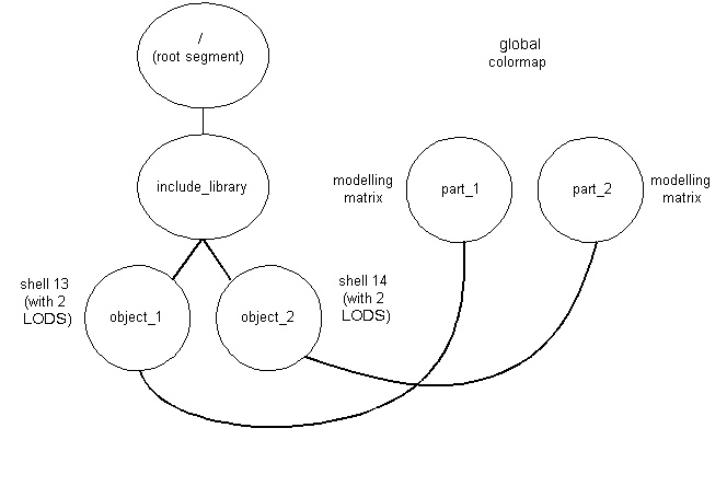
Since the main segment tree references other segments (each reference is denoted by a #TKE_Include_Segment opcode), the segments in the ‘include library’ must come first in the file. Typically, it is desirable to have any LOD representations read in first so that the reading application (which may be incrementally streaming in the data) can quickly provide a rough depiction of the scene. Therefore, we need to store LOD representations of shells at the beginning of the file. The HOOPS/Stream Toolkit supports the concept of tagging, which enables the developer to first output a LOD representation of the shell, and then later output another LOD representation (or the full representation) of that same shell and associate back to the original shell. If you want to be able to maintain this association during reading, you must follow tagging procedures which are discussed later, in Tagging HSF objects. Since the graphical information is coming from a custom set of data structures, you will need to provide your own LOD representations for shells.
Please note that LOD support could still be leveraged in the case where you are manually creating an HSF file, where you could call the utility function HC_Compute_Optimized_Shell to generate LODs.
The following is one possible structure of the HSF file which represents the above scene-graph and orders the various representations of the shell primitives:
<TKE_Comment>
<TKE_File_Info>
<TKE_View>
<TKE_Start_Compression>

<TKE_Color_Map>

<TKE_Open_Segment>                // /include_library/object_1 segment
<TKE_Shell>                       // id=13, LOD 2 - output LOD 2
<TKE_Close_Segment>

<TKE_Open_Segment>                // /include_library/object_2 segment
<TKE_Shell>                       // id=14, LOD 2 - output LOD 2
<TKE_Close_Segment>

<TKE_Open_Segment>                // part_1 segment
<TKE_Include_Segment>             // include the object_1 segment
<TKE_Modelling_Matrix>            // give it a unique mod matrix
<TKE_Color_RGB>                   // apply a local color
<TKE_Close_Segment>

<TKE_Open_Segment>                // part_2 segment
<TKE_Include_Segment>             // include the object_2 segment
<TKE_Modelling_Matrix>            // give it a unique mod matrix
<TKE_Close_Segment>

<TKE_Shell>      // id=13, LOD 1  -  output LOD 1 for the shells
<TKE_Shell>      // id=14, LOD 1

<TKE_Shell>      // id=13, LOD 0  -  output LOD 0 which is the original
<TKE_Shell>      // id=14, LOD 0

<TKE_Close_Segment>

<TKE_Stop_Compression>
<TKE_Termination>
The code required to create this HSF is simple_hsf3.cpp. Note how the example reuses opcode handlers in cases where more than one object of a specific type is going to be exported to the HSF file.
Non-Shell LODs
The LOD representation for a shell object is not restricted to a shell, but can be composed of one or more non-shell objects. For example, a circle or several polylines could be used as the LOD representation for a shell.
This is achieved by calling the TK_Shell::AppendObject method for each primitive to be used as part of the non-shell LOD representation. This would be called during initialization of the TK_Shell data (typically performed within the Interpret method) TK_Shell::AppendObject does not make any copies of the object passed into it; it only stores a pointer to objects. Therefore, all objects need to be manually cleaned up before using the shell opcode handler again, or when deleting the object. TK_Shell::PopObject should be used to obtain the pointer to the next object and remove it from the shell handler’s list of LOD objects.
The sample code reviewed above includes an example of using a non-shell LOD (a circle) to represent LOD level 2 of the shell. Note that clean up of the non-shell LOD object(s) is performed within the overwritten Reset method, which calls the base class’ Reset method. This ensures that when the shell opcode handler is reset, everything will be properly cleaned up before the opcode handler object is reused. The sample code performs clean up of the non-shell LOD objects in the Reset method instead of an overloaded constructor method because it reuses the custom shell opcode handler.
Writing Examples
We’ve seen examples of how to export several opcodes to an HSF file. Most opcodes are ‘self-contained’, and it is fairly easy to see how to initialize them by looking at the definition of the associated opcode-handler class. The protected data members must be initialized, and public functions are provided for doing so. However, some graphical attributes are more complicated in that they require export of several opcodes. Additionally, the ultimate goal is to export an existing scene-graph, and this requires familiarity with higher-level organization concepts. This section will cover these more complex situations and will evolve over time.
Sample Scene Graphs
The HOOPS/3dAF documentation contains a sample scene graph section which reviews how to design HOOPS/3dGS scene-graphs for a variety of application types. Even though it reviews use of HOOPS/3dGS to create in-memory scene-graphs, a corresponding HSF (exported using the BaseStream classes of HOOPS/Stream) would have a similar organization. Just remember that an HSF is essentially a binary archive of a HOOPS/3dGS scene-graph. The goal is to figure out what HSF opcodes to use to represent each object in the scene-graph (either a segment, a geometry primitive, or an attribute). Each of the sample scene graphs has a corresponding BaseStream sample program located in <hoops>/dev_Tools/base_stream/examples/sample_scene_graphs. A list of the sample scene graphs and their corresponding BaseStream HSF-export example are as follows:
- AEC/GIS/ECAD: base_stream_2d.cpp
- 2D/3D: base_stream_2d+3d.cpp
- CAE: base_stream_cae.cpp
- 3D/MCAD: this scene-graphs example is addressed by the simple_hsf3.cpp example at (<hoops>/dev_tools/base_stream/examples/simple/simple_hsf3.cpp).
Complex Graphical Attributes
One of the more complex graphical attributes is textures. Recalling that HSF objects are essentially archives of HOOPS/3dGS scene-graph objects, it is useful to review how texture-mapping works in HOOPS/3dGS. First, an image must be defined. Then, a texture must be defined which refers to that image. The color of the faces of a shell (or mesh) must be set to the texture name, and finally, the vertex parameters must be set on the vertices of the shell (which map into the texture).
To export this info to an HSF file, the following opcodes must be exported:
TK_ImageTK_Texture(this must be exported afterTK_Image, since it refers to it)TK_Color(this must be exported afterTK_Texture, since it refers to it)
An example of how to export a shell with a texture applied is located here and at (<hoops>/dev_tools/base_stream/examples/simple/simple_hsf4.cpp).
More Code Samples
The following is a list of samples of how various HOOPS features can be implemented using the base stream toolkit:
- decal_textured_nurbs.cpp shows a decal texture on a NURBS surface using the base stream toolkit.
- multitexture.cpp shows the use of multiple textures with the base stream toolkit.
- natural_textured_NURBS.cpp shows natural texture parameterization on a NURBS surface using the base stream toolkit.
- sectioned_cutting_planes.cpp shows sectioned cutting planes using the base stream toolkit.
- set_ambient_light.cpp shows how to set the ambient light component of a light using the base stream toolkit.
Write Options
The HOOPS/Stream Toolkit supports a variety of compression and streaming options which are used when exporting an HSF file. It may be desirable to modify these settings based on how your model is organized, the size of the model, and the amount of preprocessing time that is acceptable.
Write options are set on the toolkit by calling BStreamFileToolkit::SetWriteFlags. File write options are specified by #TK_File_Write_Options enumerated type in BStream.h.
When using the base classes to manually map graphics information to an HSF file, only a subset of the file-write-options are supported, and the details are listed in each of the option descriptions below:
| Supported | Unsupported |
|---|---|
#TK_Full_Resolution_Vertices |
#TK_Suppress_LOD |
#TK_Full_Resolution_Normals |
#TK_Disable_Priority_Heuristic |
#TK_Full_Resolution |
#TK_Disable_Global_Compression |
#TK_Force_Tags |
#TK_Generate_Dictionary |
#TK_Connectivity_Compression |
#TK_First_LOD_Is_Bounding_Box |
Those in the “unsupported” column are there because they only make sense in the context of a specific graphics system, and dictate overall file organization. (They are supported by the ‘3dgs’ classes) Users of the base classes are free to implement them (or not implement them), according to the needs of their application. All bits are by default off (set to zero). The following reviews the various types of options, along with their default values and usage:
Compression During Writing
Global Compression The toolkit performs LZ compression of the entire file using the zlib library. This is a lossless compression technique that permits pieces of the compressed file to be streamed and decompressed, and is computationally efficient on both the compression and decompression sides.
Usage: off by default; needs to be manually enabled by exporting #TKE_Start_Compression and #TKE_Stop_Compression opcodes to the file. Setting #TK_Disable_Global_Compression will have no effect.
The HOOPS/Stream Toolkit will also compress raster data by default, using a JPEG compression utility. The compression level of this data can be controlled by calling BStreamFileToolkit::SetJpegQuality.
Geometry compression
Geometry compression is currently focused on the ‘shell’ primitive, (represented by the #TKE_Shell opcode, and handled by the TK_Shell class) This is the primary primitive used to represent tessellated information. Datasets typically consist primarily of shells if the data sets originated in MCAD/CAM/CAE applictions.
A TK_Shell object has local write sub-options which may or may not reflect the directives from the BStreamFileToolkit object’s write options. A public function, TK_Shell::InitSubop is available to initialize the write sub-options of TK_Shell with the BStreamFileToolkit write options. You should set up your desired write options on the BStreamFileToolkit object, and then call InitSubop within your shell opcode-handler’s constructor or Interpret function. The shells’ local sub-options may also be directly modified by calling TK_Shell::SetSubop, and passing in any combination of the options enumerated in TK_Polyhedron.
Vertex compression - This involves encoding the locations of shell vertices, providing reduction in file size in exchange for loss of coordinate precision and slightly lower visual quality. The degradation in visual quality is highly dependent on the topology of the shell, as well as how the normals information is being exported. The function BStreamFileToolkit::SetNumVertexBits allows the developer to control the number of bits of precision for each vertex. The default is 24 (8 each for x, y and z).
Usage: Enabled by default within the BStreamFileToolkit object. Disabled by setting #TK_Full_Resolution_Vertices and/or #TK_Full_Resolution.
Usage is controlled at the local shell level by calling TK_Shell::SetSubop and using the TKSH_COMPRESSED_POINTS define. For example, to turn this on, you would call SetSubop(``TKSH_COMPRESSED_POINTS | GetSubop()) To turn this off, you would call SetSubop(~TKSH_COMPRESSED_POINTS & GetSubop())
Normals Compression - Normals will be automatically exported to the HSF file if normals were explicitly set on geometry using the TK_Polyhedron::SetFaceNormals(), TK_Polyhedron::SetEdgeNormals(), or TK_Polyhedron::SetVertexNormals(). Normals compression involves encoding vertex normals, providing reduction in file size in exchange for lower visual quality. Again, the degradation in visual quality is highly dependent on the topology of the shell, as well as how the normals information is being exported. HOOPS/Stream transmits compressed normals for vertices that have been compressed, or if a normal has been explicitly set on a vertex. Surfaces that had gradual curvature over a highly tessellated region can look faceted due to the aliasing of the compressed normals. The function BStreamFileToolkit::SetNumNormalBits allows the developer to greatly reduce or effectively remove such aliasing at the cost of transmitting more data per normal. The default is 10.
Usage: Enabled by default within the BStreamFileToolkit object. Disabled by setting #TK_Full_Resolution_Normals and/or #TK_Full_Resolution.
Usage cannot currently be controlled at the local shell level.
Parameter compression - This involves encoding the vertex parameters (texture coordinate). Compression will reduce the file size but this could also result in the loss of precision in textures mapping.
Parameter compression is on by default, and can be disabled by setting the #TK_Full_Resolution_Parameters bit in the flags parameter.
The function HStreamFileToolkit::SetNumParameterBits allows the developer to control the number of bits of precision for each vertex. The default is 24 per component.
Connectivity compression - This compresses ‘shell’ connectivity information. This compression technique can provide compelling reductions in files sizes for datasets that contain many ‘shell’ primitives, but can also be a computationally intensive algorithm depending on the size of individual shells. Developers will need to decide for themselves whether the reduced file size is worth the extra computation time.
Additionally, depending on the topology of the shell, the algorithm may provide limited compression benefit or have to ‘punt’ after performing substantial work, thereby providing little to no additional file size reduction in exchange for extra computation time. Therefore, developers should do some experimentation with their specific class of datasets to see if the option is buying them any reduction in file size. If files sizes for typical files are the same both with and without the option set, then this compression option should be disabled when exporting an HSF file. Some specific examples of when the algorithm will punt or perform poorly are shells that contain many backwards faces (which also impact rendering performance and should generally be avoided anyway!), or contain certain complex combinations of ‘handles’ ( a teapot or a torus each have one handle) and holes (i.e. a flat plate that has a hole in the middle). In general, the connectivity compression algorithm will perform well with most of these cases, but developers should still take some time to investigate the [extra export time vs. file-size reduction] of their datasets with and without this option enabled.
Usage: Disabled by default within the BStreamFileToolkit object. Enabled by setting #TK_Connectivity_Compression.
Usage is controlled at the local shell level by calling TK_Shell::SetSubop and using the TKSH_CONNECTIVITY_COMPRESSION define. For example, to turn this on, you would call SetSubop(TKSH_CONNECTIVITY_COMPRESSION | GetSubop()) To turn this off, you would call SetSubop(~TKSH_CONNECTIVITY_COMPRESSION & GetSubop())
Dictionary
Part of the HSF specification is a “dictionary” of file offsets. Its main purpose is to allow selective refinement of graphic database detail. The 3dgs classes will write such a dictionary at the end of the file if the #TK_Generate_Dictionary write option is set. Though it would also be possible to create a dictionary with the base classes, there is not yet a public interface to do so. Users of the base classes who would like to take advantage of this area of the HSF specification should contact technical support.
LOD Options
Three of the file write options (#TK_Suppress_LOD, #TK_First_LOD_Is_Bounding_Box, and #TK_Disable_Priority_Heuristic) control the existence and/or appearance of levels of detail. As with geometry compression (see above), these options are currently geared towards the TK_Shell opcode.
#TK_First_LOD_Is_Bounding_Box: as the name suggests, this option causes the first LOD of any shell to be replaced with its axis aligned bounding box. The final argument toTK_Shell::InitSubopis a boolean, is_firstpass. The shell is replaced with its bounding box only if the write option#TK_First_LOD_Is_Bounding_Boxand the is_firstpass argument toTK_Shell::InitSubopare set.#TK_Suppress_LODand#TK_Disable_Priority_Heuristicare not supported and will not have any effect on the HSF contents written by base_stream. If they are to be respected at all, they are completely the user’s responsibility.#TK_Suppress_LODis meant to prevent any levels of detail from getting into the file.#TK_Disable_Priority_Heuristic, will indicate not to sort detail levels according to some heuristic that weighs cost versus benefit – putting the most important things first.
Tagging
The toolkit supports the concept of tagging, discussed in this section Setting #TK_Force_Tags will cause tags to be automatically generated by the toolkit during the writing process. (Note: tags will always be generated for shells regardless of the value of this write option.)
Global Quantization
Setting #TK_Global_Quantization will cause any required quantization to be global (bbox of scene) instead of local (bbox of individual geometry) . This is useful for situations where high-level objects are split up into multiple shells, since it avoids cracks between the sub-objects (Using a solid modeling example, this would be a situation where a shell was used for each ‘face’, instead of using a single shell for each higher-level ‘body’.) Regardless of this flag, however, local quantization applies until the first #TKE_Bounding_Info. This flag is off by default.
Exporting Different HSF Versions
When writing information out to an HSF file, you will want to indicate what version the file is written in. To specify this information, use the method BStreamFileToolkit::SetTargetVersion. Then pass an integer indicating the file version. For instance, if you want to export a version 16.00, you would pass the integer 1600 when calling BStreamFileToolkit::SetTargetVersion. The following code snippet shows how you would indicate what version of HSF you are exporting:
//setup the toolkit to export v15.00 HSF File
my_toolkit->SetTargetVersion(1500);
The default value for the target version is the most recent version in the file version table.