Computing Ambient Occlusion

Ambient occlusion offers an important visual clue helping to understand how the model is setup. Refer to the Tracing Custom Rays tutorial for all details on how an ambient occlusion is being calculated. The process followed in this book is more or less a copy / paste of the tutorial’s contents.

Pre Processing Ambient Occlusion

• We start parsing the scene graph and concatenate the current matrix transform to perform all calculations in world space.

// Recursive parsing of our scene graph:
// -------------------------------------

if( itshape )
{
    int i, count;
    RED::Object* child;
    RED::Matrix matx;
    const RED::Matrix* tmatx;

    RC_TEST( itshape->GetMatrix( tmatx ) );
    matx = ( tmatx ) ? *tmatx : RED::Matrix::IDENTITY;

    RED::Matrix mlast = ( mstack.empty() == false ) ? mstack.back() : RED::Matrix::IDENTITY;
    RC_TEST( mstack.push_back( mlast * matx ) );

    RC_TEST( ishape->GetChildrenCount( count ) );
    for( i = 0; i < count; i++ )
    {
        RC_TEST( ishape->GetChild( child, i ) );
        RC_TEST( AmbientOcclusionSetup( child, mstack, geometry_db, parsed_vertices_count, vertices_count ) );
    }

    mstack.pop_back();
}

• Then we add one vertex channel to the geometry, that will store the calculated ambient occlusion factor.

RC_TEST( imesh->GetVerticesCount( count ) );
RC_TEST( imesh->GetVertexArray( (const void*&)vertex, vsize, vformat ) );
RC_TEST( imesh->GetNormalArray( (const void*&)normal, nsize, nformat ) );

RC_TEST( imesh->SetArray( RED::MCL_TEX0, NULL, count, 1, RED::MFT_FLOAT, iresmgr->GetState() ) );
RC_TEST( imesh->GetArray( (void*&)ao, RED::MCL_TEX0, iresmgr->GetState() ) );

• Finally we can visualize our result if we tweak the display shader a little bit, just to visualize “ao.x” in “result.color”:

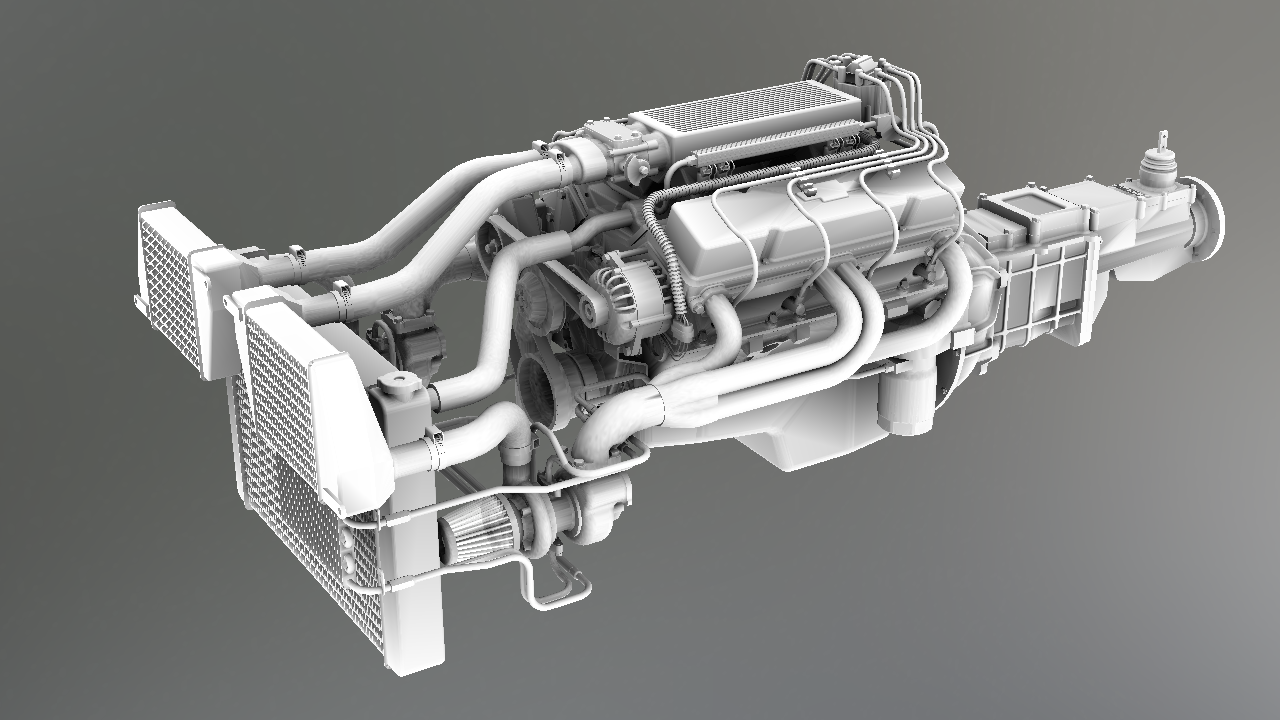
The ambient occlusion layer displayed standalone

In a classic CAD assembly, the ambient occlusion layer has a varying quality depending on how the underlying tessellation is performed. As the ambient occlusion term is stored in a vertex channel, it’s submitted to interpolation along a triangle. In CAD models, we have a lot of long thin triangles that are set to minimize the total number of triangles in the resulting mesh. If one vertex has a dark ambient occlusion and one other a bright ambient occlusion, we’ll see the interpolation between the two values, as pointed out in the close-up below:

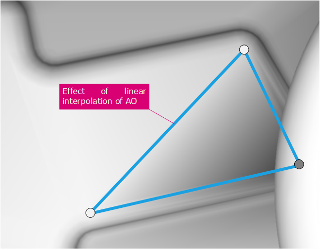
Interpolation artifacts resulting of a raw ambient occlusion

In this example, one triangle vertex is hidden by the pipe above it, so it has a quite dark ambient occlusion factor. As a consequence, this leaks during the interpolation process along the triangle of the hardware rasterizer.

Modulating Skylight and Environmental Lighting Contribution

// Skylight contribution:
str.Temp( "ao" );
str.Temp( "ao_color" );
str.Add( "MOV ao, fragment.texcoord[3];\n" );
str.SkylightDiffuseLighting( "ao_color", "normal", NULL, "texture[2]" );
str.Add( "MUL ao_color, ao_color, ao.x;\n" );
str.Add( "MUL ao_color, ao_color, diffuse_color;\n" );
str.Add( "MUL env_color, env_color, ao.x;\n" );

The AO contribution is then used to modulate a skylight contribution:

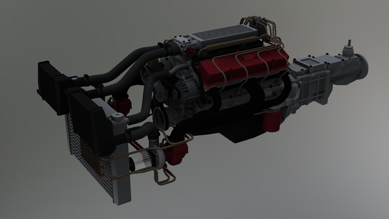
The AO value modulating the skylight lighting.

And the environmental lighting. This attenuates the fact that environmental lighting is lacking self shadows of the object reflections on itself:

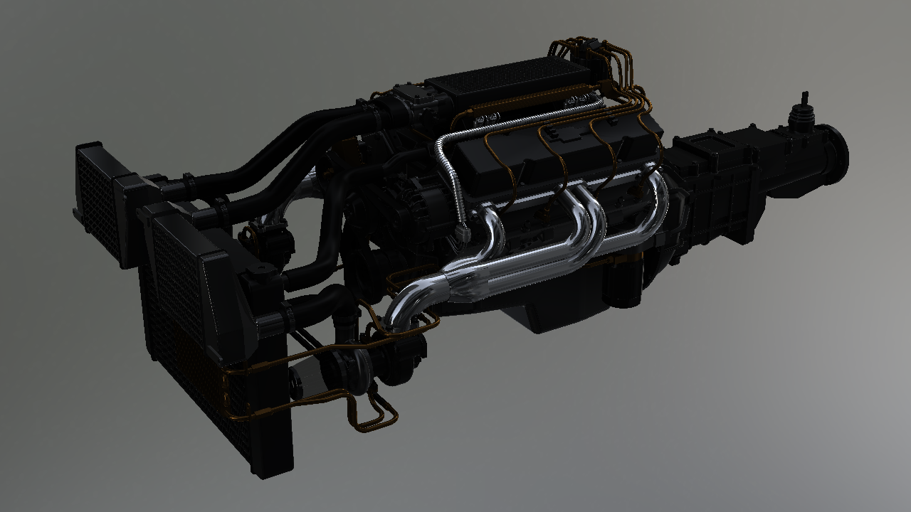
The AO value modulating the environmental lighting.