Volume View

Introduction

This tutorial shows an example of creation and display of a 3D image. The program loads a Computed Tomography dataset (CT scan) from the disk and generates a 3D texture out of it. The skull scan information was downloaded from www.volvis.org.

Because 3D images are not easy to visualize, we detail a rendering method based on slice planes drawing.

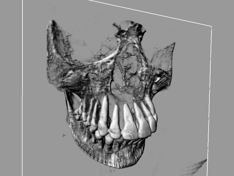
The scanner dataset visualized with planar slices

Creating a 3D Image

3D images are created like all other kind of images, through the RED::IResourceManager interface. Then the RED::IImage3D interface provides the needed access to the image’s specific properties:

RED::Object* image3D;
RC_TEST( iresmgr->CreateImage3D( image3D, iresmgr->GetState() ) );
RED::IImage* iimage = image3D->As< RED::IImage >();
RED::IImage3D* iimage3D = image3D->As< RED::IImage3D >();

RC_TEST( iimage3D->SetPixels( pix, RED::FMT_RGBA,RED::TGT_TEX_3D, 256, 256, 256, iresmgr->GetState() ) );
RC_TEST( iimage3D->SetWrapModes( RED::WM_CLAMP_TO_BORDER,
                                RED::WM_CLAMP_TO_BORDER,
                                RED::WM_CLAMP_TO_BORDER, iresmgr->GetState() ) );
RC_TEST( iimage->SetFilterModes( RED::FM_LINEAR, RED::FM_LINEAR, iresmgr->GetState() ) );

As we’re now using three coordinates for the sampling of the texture in a pixel shader program, we need a specific method to specify the 3rd coordinates wrapping mode. RED::IImage3D::SetWrapModes redefines the 2D images method specifically for 3D images.

3D images may be created as Power-Of-Two-Dimensioned (POTD) or Non-POTD. Both are possible. However, unlike 2D images, the sampling coordinates used for the texture access always must remain in the [0, 1] x [0, 1] x [0, 1] unit cube, this both for POTD and NPOTD images.

Slice Based Visualization

The slice based rendering method uses view plane aligned polygons covering the 3D image’s area to perform a slicing of the volume to render. The schema below illustrates that:

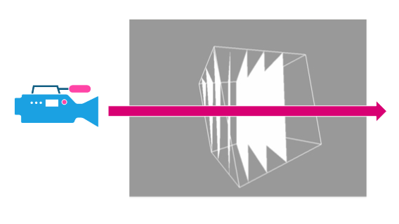
Slice visualization using view aligned polygons

Polygons are created perpendicular to the camera sight vector and clipped by the volume boundaries (the cube in our example). Then, a back to front rendering of all the polygons is performed using a custom shader and a blending equation based on the scanner density information. The volume reconstruction effect arises when the number of slices is high enough to fake a dense volume effect:

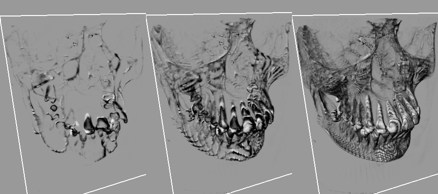
From left to right: 10, 40 and 128 slices in the rendering

When only 40 slices are used for the rendering, we clearly see the banding effects: 40 parallel planes are not enough to simulate the volume effect. The application is set initially to 256 planes. Increasing that number will add more quality, and make close-up views look nicer. Note that we use a non linear slice distribution in the sample to get more slices close to the camera than far from it.

Shading and Lighting Volumic Data

Shading is a real problem with volume datasets, as we have no defined geometry and no surface for it. If we simply output the input opacity we don’t get a good result. If we apply a transform curve (a bell curve in the sample) to focus on a given density, then the result looks better:

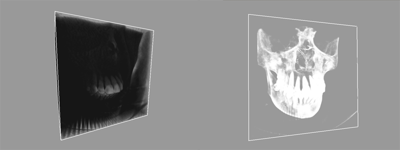
Input opacity as output on the left, filtered opacity output on the right

However, without local surface normal information, we can’t get a surface feeling, as there’s no lighting information to play with.

This is why we introduce a local surface normal through a simple gradient computation. This has a key advantage as this can be used to apply all standard lighting equations to the shader: diffuse lighting, specular lighting, reflection vectors, etc…

We store this normal in the XYZ fields of the 3D texture. The main drawback of that operation is that we use 4 times more memory than if we were to only store the density on an 8 bit value. We’ll discuss this issue in the next paragraph.

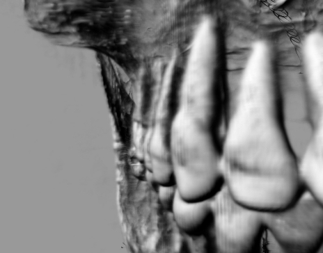
Close-up view on the lighting model.

Visualizing Larger Datasets

The dataset we have visualized was containing 256 x 256 x 256 x 8 bit voxel information. This information alone uses more than 16 Mb of video RAM. If we were to display a 512 x 512 x 512 dataset, then the consumed memory would climb to 128 Mb of video memory.

Adding normals to the volume information is useful for all lighting calculations, but this increases our memory usage a lot, making it difficult to visualize large datasets. Therefore, we need to implement some kind of compression schema here to save memory.

Normal Compression

A first easy optimization can be performed on the memory used to store local normals: we can reduce normals accuracy to 16 bits.

Normals stored on 16 bits can use a 6 x 5 x 5 sampling or a polar coordinates encoding to sample all possible directions. Then a simple table using a 256 x 256 lookup texture can be used to reconstruct the normal from its 16 bits encoding.

This saves 25% of the memory used for the storage of the 3D texture. In that case, a RED::FMT_RGB format texture can be created instead of a RED::FMT_RGBA texture.