Sketch Rendering

Introduction

Sketch rendering is often used to give a more natural or artistic look to synthetic images. It focuses the attention of the viewer on shapes and colours and is useful for design projects like architectural projects, object manufacturing, etc.

In this tutorial we demonstrate how to achieve such a rendering style with HOOPS Luminate, easily. Because of the number of stages in the process of sketch rendering, we chose to separate the whole thing into two distinct parts for readability.

This part is involved in producing two images: a RGB image and an edges image. Both images are then used in the second part of the tutorial to render the full scene with sketch look.

Rendering the RGB and Contours Images

We start from an external .red file. This lets you replace the provided .red file with your own to check the sketch effect on your data. Because of the simplicity of the default input scene, rendering options are set to quite low values: only four levels of reflection are set. Following the rule which says that ray-traced shadows depth must be greater than those for reflections and refractions, we set the shadow depth to 5 (this ensures that shadows are also visible through reflections and refractions).

Finally, tone mapping is turned on to ensure that, whatever the input data are, something well-exposed will be rendered. Check Tone Mapping for more information about post processing in HOOPS Luminate.

// Load the scene.
RED::Object* camera;
unsigned int context;
RC_TEST( app::LoadREDFile( camera, context, NULL, "../resources/conference.red" ) );

RED::IViewpoint* icamera = camera->As< RED::IViewpoint >();

// Set the rendering options.
RED::IOptions* icamopt = icamera->As< RED::IOptions >();
RC_TEST( icamopt->SetOptionValue( RED::OPTIONS_RAY_GI, true, iresmgr->GetState() ) );
RC_TEST( icamopt->SetOptionValue( RED::OPTIONS_RAY_PRIMARY, true, iresmgr->GetState() ) );
RC_TEST( icamopt->SetOptionValue( RED::OPTIONS_RAY_REFLECTIONS, 4, iresmgr->GetState() ) );
RC_TEST( icamopt->SetOptionValue( RED::OPTIONS_RAY_REFRACTIONS, 4, iresmgr->GetState() ) );
RC_TEST( icamopt->SetOptionValue( RED::OPTIONS_RAY_TRANSPARENCY, 4, iresmgr->GetState() ) );
RC_TEST( icamopt->SetOptionValue( RED::OPTIONS_RAY_SHADOWS, 5, iresmgr->GetState() ) );

RC_TEST( icamopt->SetOptionValue( RED::OPTIONS_RAY_LIGHTS_SAMPLING_RATE, 3, iresmgr->GetState() ) );
RC_TEST( icamopt->SetOptionValue( RED::OPTIONS_RAY_GLOSSY_SAMPLING_RATE, 3, iresmgr->GetState() ) );

RC_TEST( icamera->GetPostProcessSettings().SetToneMapping( RED::TMO_PHOTOGRAPHIC ) );

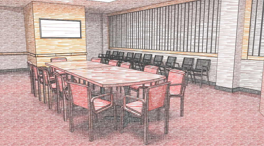
The scene is rendered a first time to produce the RGB image. Then, we slightly change the rendering set up to render the contours image.

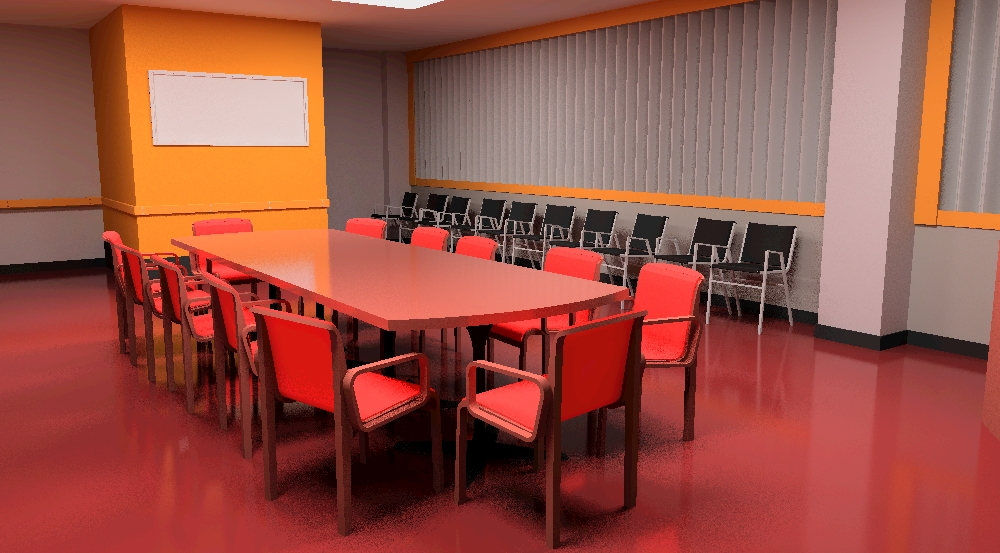
The RGB image produced by the tutorial.

The most complicated part of the tutorial is perhaps the correct rendering of edges. HOOPS Luminate exposes everything needed to do that, but data need a little bit of set up.

First, we create two materials: one for the edges and one for the geometry. That’s because we want to render the edges in a given colour while rendering the geometry in white to hide it. Moreover, we need to apply some polygon offset to the geometries to avoid any overlapping between geometries and edges.

RC_TEST( iresmgr->CreateMaterial( matr_edges, state ) );
RED::IMaterial* imatr = matr_edges->As< RED::IMaterial >();

RED::StateShader state_shader;
RC_TEST( state_shader.SetLineWidth( 6.f ) );

RC_TEST( imatr->RegisterShader( state_shader, state ) );
RC_TEST( imatr->AddShaderToPass( state_shader.GetID(), RED::MTL_PRELIT, RED::LIST_LAST, RED::LayerSet::ALL_LAYERS, state ) );

RED::RenderShaderEdges shedges( RED::MTL_PRELIT,
                                RED::MCL_VERTEX,
                                RED::MCL_USER0,
                                RED::MCL_USER1,
                                RED::Color::BLACK,
                                true,
                                true,
                                RED_PI,
                                resmgr, rc );
RC_TEST( rc );

RC_TEST( imatr->RegisterShader( shedges, state ) );
RC_TEST( imatr->AddShaderToPass( shedges.GetID(), RED::MTL_PRELIT, RED::LIST_LAST, RED::LayerSet::ALL_LAYERS, state ) );

The first material is the edges material. A RED::StateShader is used to set up the style of the edges. The RED::RenderShaderEdges is a built-in rendering shader which is used to dynamically render contour and border edges.

The second material is the geometries material and is made, once again, of two shaders:

RC_TEST( iresmgr->CreateMaterial( matr_geo, state ) );
imatr = matr_geo->As< RED::IMaterial >();

RED::StateShader ss;
RC_TEST( ss.SetPolygonOffset( true ) );
RC_TEST( ss.SetPolygonOffsetValue( 1.0f, 1.0f ) );

RC_TEST( imatr->RegisterShader( ss, state ) );
RC_TEST( imatr->AddShaderToPass( ss.GetID(), RED::MTL_PRELIT, RED::LIST_LAST, RED::LayerSet::ALL_LAYERS, state ) );

RED::RenderShaderSolid white( RED::MTL_PRELIT, RED::Color::WHITE, NULL, RED::Matrix::IDENTITY, RED::MCL_TEX0,
                              RED::Color::WHITE, NULL, RED::Matrix::IDENTITY, RED::MCL_TEX0, resmgr, rc );
RC_TEST( rc );

RC_TEST( imatr->RegisterShader( white, state ) );
RC_TEST( imatr->AddShaderToPass( white.GetID(), RED::MTL_PRELIT, RED::LIST_LAST, RED::LayerSet::ALL_LAYERS, state ) );

The RED::StateShader is used to set up polygon offset. This ensures that geometries will be drawn a little bit away from the edges to avoid overlapping and z-fighting effect. The RED::RenderShaderSolid is set to constant white to make the geometries disappear in the background. That’s because we are only interested in the edges for that rendering.

The very last thing to do is to build the edge geometries. This must be done for any mesh in the scene.

First, the list of scene meshes is built. Starting from the scene root, we look for every scene graph node implementing the RED::IMeshShape interface:

RED::IShape* iroot = root->As< RED::IShape >();

RED::Map< RED::Object*, unsigned int > meshes;
RC_TEST( iroot->GetShapes( meshes, RED::IMeshShape::GetClassID() ) );

Once done, we loop over those meshes to call RED::IMeshShape::BuildContourEdges on each:

for( meshes.begin(); !meshes.end(); meshes.next() )
{
  RED::IMeshShape* imesh = meshes.current_key()->As< RED::IMeshShape >();

  // Before building the edges, we clean the mesh a little bit by collapsing
  // its vertices which are close enough from each others.
  RED::Vector< RED::MESH_CHANNEL > tol_dist, tol_angle;

  // Cleaning is performed by collapsing the mesh vertices based only on position
  // and normals similarities.
  RC_TEST( tol_dist.push_back( RED::MCL_VERTEX ) );
  RC_TEST( tol_angle.push_back( RED::MCL_NORMAL ) );
  RC_TEST( imesh->Collapse( 1e-5, 0.01, state, &tol_dist, &tol_angle ) );

  // We can now build the contour edges.
  RED::Object* contour;
  contour = RED::Factory::CreateInstance( CID_REDLineShape );
  if( contour == NULL )
    return RED_ALLOC_FAILURE;

  RC_TEST( imesh->BuildContourEdges( contour,
                                    RED::MCL_VERTEX,
                                    RED::MCL_USER0,
                                    RED::MCL_USER1,
                                    RED::MCL_VERTEX,
                                    state ) );

Before calling RED::IMeshShape::BuildContourEdges, we clean the meshes by calling RED::IMeshShape::Collapse.

This call merges vertices which are below some user-defined thresholds. Those thresholds are about proximity in space or orientation and can be set for any mesh geometry channel. Here, we chose to weld vertices based only on their positions and normals.

We then assign our two previously created materials to the edges and scene geometries:

// Assign the contour material to the contour geometry.
RED::IShape* icshape = contour->As< RED::IShape >();
RC_TEST( icshape->SetMaterial( matr_edges, state ) );

// Assign the white material to the geometries.
RED::IShape* ishape = meshes.current_key()->As< RED::IShape >();
RC_TEST( ishape->SetMaterial( matr_geo, state ) );

To end the scene setup process, we link the new contour geometries to the same parents than those of the geometries they are extracted from:

// Add the contour geometry to the scene graph.
const RED::Vector< RED::Object* >* parents;
RC_TEST( ishape->GetParents( parents ) );

for( unsigned int p = 0; p < parents->size(); ++p )
{
  RED::ITransformShape* iparent = (*parents)[p]->As< RED::ITransformShape >();
  RC_TEST( iparent->AddChild( contour, RED_SHP_DAG_NO_UPDATE, state ) );
}

The scene set up is now over.

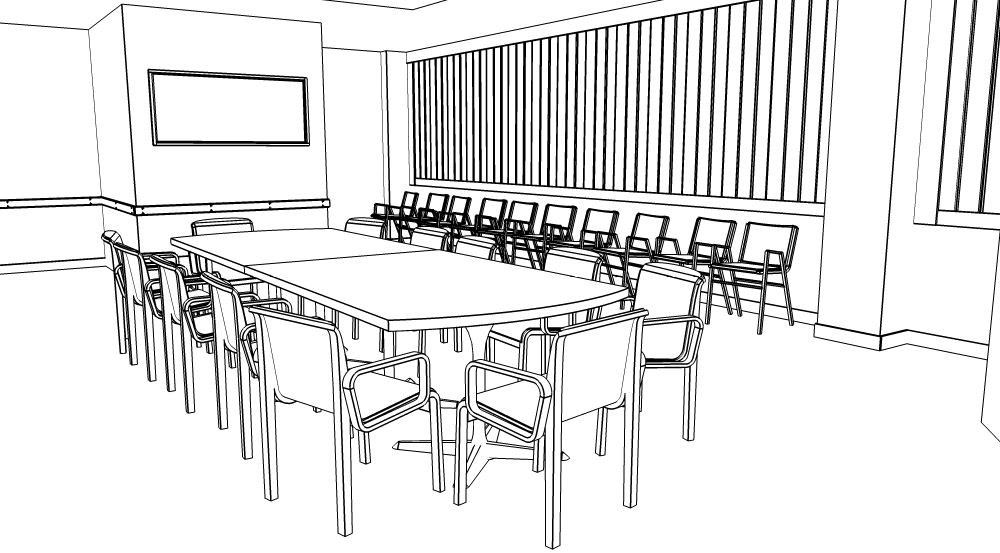
The contours image produced by the tutorial.

Rendering the Sketch Effect

We decided to implement a screen-space sketching algorithm due to major advantages:

• The scale of the strokes is uniform over surfaces: whatever the distance to surfaces from the eye is, pencil strokes have a constant width

• The sketch shading does not depend on geometry materials; therefore the latter don’t have to be modified to support sketch rendering

• A single shader has to be written and kept updated as it is applied to the whole screen at once

The Sketch Rendering Algorithm

There are plenty of ways to do sketch rendering. We chose one which gives very fast, easy to setup, nice results. We use a set of 4 hand-drawn stroke textures. Each one is seamless and represents a shading level (ranging from light to dark grey).

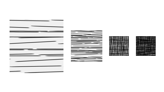
The four stroke textures used to render sketch pictures.

The algorithm proceeds as follows:

• For each pixel of the RGB input image, the average over the color components is computed (kind of gray level)

// Compute the gray level of the rgb color in [0, 1]...
double brightness = REDMax<double>( 0.0, REDMin<double>( 1.0, ( rgb[0] + rgb[1] + rgb[2] ) / 3.0 ) );

• The opposite of the level computed in 1. is quantized to one of four gray levels (from 0 to 3); we take the opposite because drawing, just as printing, is a subtractive color operation: brightest areas are those where the paper (most often white) is the most visible

// and invert it! We assume that the paper on which the drawing is performed is bright.
// So we have to think to our painting process as a subtractive color operation.
brightness = 1.0 - brightness;

// We allow only four levels of shading in the drawing (through different hatching textures).
// So, we quantize the brightness into 4 different values in {0, 1, 2, 3}.
int level = (int)( brightness * 4.0 );
level = REDMin( 3, level );

• The quantification in 2. gives us the texture to use to draw the current pixel

double pencil_color[4];
rayContext.SampleTexture( pencil_color, 0, 2 + level, pencil_uv, RED::Matrix::IDENTITY, shaderContext, renderingContext );

• The destination pixel is written using the texture selected in 3. multiplied by the input RGB pixel color; the mapping of the texture is done screen-space, i.e pixel coordinates are used to address the texture texels (repeat tiling is set to four textures). The pencil color is blended with the paper one:

// Blend the edge and pencil strength together. The edges take over the pencil strength as
// we want to clearly see our edges in the final result.
//
//                [ edge strength ]   [    pencil strength    ]
//                |||||||||||||||||   |||||||||||||||||||||||||
pencil_strength = ( 1.0 - edge[0] ) + edge[0] * pencil_strength;

Here is what we get if we use only the first stroke texture for shading.

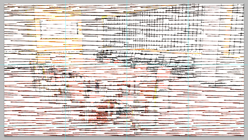
The image rendered using only the first stroke texture.

As you can see, the texture (which is 256x256) is repeated over the whole screen to cover the input image resolution. This is not sufficient to give the exact feeling about lighting and materials. That’s why we select one of our 4 different stroke textures in every pixel.

The same image rendered using four stroke textures.

To enhance the object shapes, we use the input edges image. To do so, we ensure that edges will be visible by blending giving them the priority over the pencil computed from the colour:

double cr = paper_color[0] * ( 1.0 - pencil_strength ) + rgb[0] * pencil_strength;
double cg = paper_color[1] * ( 1.0 - pencil_strength ) + rgb[1] * pencil_strength;
double cb = paper_color[2] * ( 1.0 - pencil_strength ) + rgb[2] * pencil_strength;

When edges are present, i.e edge[0] is 0.0, the pencil strength is forced whatever the RGB input image is. This has the effect of making the edges always visible.

Porting the Algorithm to the GPU

Due to its simplicity, the algorithm can easily be ported to the GPU. However, some adjustments must be done to account for known GPU limitations.

We’ll focus on the main difference between CPU and GPU versions. In the CPU version, we select a stroke texture based on the brightness of the colour to reproduce. As this is quite complicated to do branching on the GPU, we must go another way with the hardware version of the shader. To do so, we use a table of four entries which maps a brightness value in [0, 3] to a 4d masking value. This can easily be done using a texture of dimensions 4x1 in RGBA format. Here is the content of the texture:

• first texel -> { 1, 0, 0, 0 }

• second texel -> { 0, 1, 0, 0 }

• third texel -> { 0, 0, 1, 0 }

• fourth texel -> { 0, 0, 0, 1 }

In the shader, we compute four pencil strengths in parallel, one for each stroke texture:

// Read the stroke texture mask from the quantization texture.
psh.Add( "MUL R0.x, R0.x, { 4.0 }.x;\n" );
psh.Add( "TEX R0, R0.xxxx, texture[6], RECT;\n" );

Then, the brightness computed by the shader is used as a 1d texture coordinate to look into the table for the right mask value:

// Extract the final pencil strength based on the stroke texture
// mask value in R0. If texture 0 should be kept, R0 = { 1, 0, 0, 0 },
// If texture 1 should be kept instead, R0 = { 0, 1, 0, 0 }, and so on...
psh.Add( "MUL pencil_strength, R0.xxxx, pencil0;\n" );
psh.Add( "MAD pencil_strength, R0.yyyy, pencil1, pencil_strength;\n" );
psh.Add( "MAD pencil_strength, R0.zzzz, pencil2, pencil_strength;\n" );
psh.Add( "MAD pencil_strength, R0.wwww, pencil3, pencil_strength;\n" );

This value is finally applied to the four stroke texture values:

pencil_strength = 0 * pencil0 + 0 * pencil1 + 1 * pencil2 + 0 * pencil3

Each pencil strength is multiplied by the corresponding entry in the mask value and added to the others. Hence, if the mask value equals { 0, 0, 1, 0 }, the shader will compute:

pencil_strength = 0 * pencil0 + 0 * pencil1 + 1 * pencil2 + 0 * pencil3

which is what we expect. For the rest of the shader, most of the program is a literal translation from C/C++ language to ARB.

Conclusion

What’s nice with this method is that you can change the input stroke textures to anything else to get totally different artistic style (dots, stains and so on).