Preparing the Point Shape Data

By default, clouds of points are rendered using a RED::IPointShape. The stored primitives are points (position and color). As seen on the page Rendering Clouds of Points: A Dynamic Point Splatting Example, rendered points have a fixed screen space size, which seems nice when viewed from a certain distance, but not so much after a zoom on the shape.

What Do We Draw?

In order to correctly see the points, they need to have a world space size instead of the 1 pixel screen size. The only way to make them thicker is to not draw points but meshes.

We have the choice about what shape to draw as a replacement of points:

• Triangle

• Square (made of 2 triangles)

• Hexagon (made of 4 triangles)

• Octagon (made of 6 triangles)

• More complex shape…

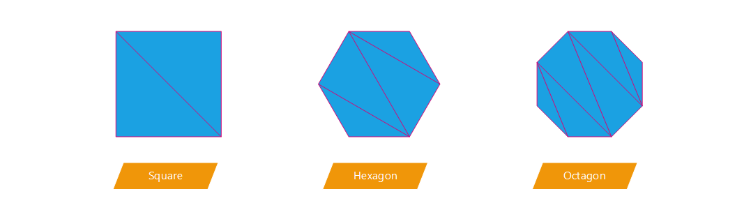
Different shapes and there triangles composition

In our application, we made the choice to test the square option as well as the octagon one. We have to keep in mind that the more complex the shape is, the more time will be taken by HOOPS Luminate to render our heavy scenes (several millions of points). As often, a choice has to be made between rapidity and rendering quality.

Note

3D shapes like sphere could also be envisaged but the number of triangles would be too high. It is highly preferable to use oriented 2D shapes to lighten the scene.

We have two solutions to transform the points in meshes:

• Creating RED::IMeshShape instead of RED::IPointShape during the scene preprocessing time and sending a mesh to the GPU;

• Sending RED::IPointShape to the GPU and creating triangles using the geometry shader at runtime.

Both options are available in the application but we will focus on the second one has it is faster and avoid sending a huge amount of primitives to the vertex shader.

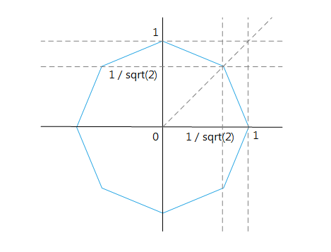
The octagon coordinates

Using the geometry shader to transform the points in octagon, here is the definition of the top right point of the octagon (let d be the shape radius):

offset = gl_ProjectionMatrix * vec4( d * invsqrt2, d * invsqrt2, 0.0, 0.0 );
gl_Position = gl_in[ 0 ].gl_Position + offset;

As you can see, the vector is in the camera space, it is multiplied by the projection matrix because the output of the geometry shader must be in clip space. The projection matrix transforms the camera space into clip/screen space.n The square version is much simpler as there are only four vertices with -d and d as coordinates.

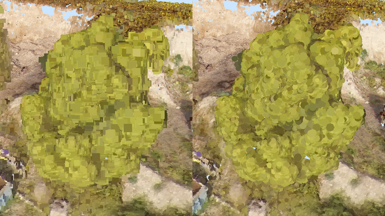
The square version of a tree (left) compared to the octagon one (right)

Another solution could have been to draw quads and to apply an opacity map on it. This would allow to render perfect circles or other more exotic shapes. This solution should be avoided because it requires transparencies. Activating transparency is very expensive and not really suitable for the real-time objective. Indeed, either transparent shapes must be sorted to be correctly rendered in real-time or the transparency have to be handled by ray-tracing.

Filling the Empty Space

Before addressing the shader topic, we need to find what will be the size of our points. The created shapes (square or octagon) have to fill the empty space between points. As the distance between points is not constant and varies from one model to another but also inside the models, the point size must be calculated for each point. Each point has to be large enough to cover the empty space around it.

Several shape radii can be tested (from smallest to largest):

• The distance between the point and his nearest neighbour

• The average distance between the point and his n neighbours

• The distance between the point and his furthest neighbour among its n neighbours

Now we see the usefulness of a good spatial data structure to retrieve the neighbours of a point (see How to Handle Efficiently the High Number of Points?).

The chosen solution is the second one: the average distance between the points and n neighbours. It is a good balance between the first one which lets too much uncovered space and the last which leads to too much overlapping.

// Computing the average distance between the point and its neighbours.
double avg_dist = 0.0;
for( int n = 0; n < neighbours.size() - 1; ++n )
{
  // '_distance2' is the square distance from the point to its neighbour.
  avg_dist += sqrt( neighbours[n]._distance2 );
}
avg_dist /= ( neighbours.size() - 1 );

// Setting the data inside the first coordinate of the texture coordinates array.
// - 'meshi' is the i-th mesh.
// - 'pti' is the i-th point of the mesh.
// - texcoord array is composed of 2 coordinates.
texcoord_out[ meshi ][ pti * 2 ] = (float)avg_dist;

For the geometry shader solution, this size information need to be sent to the shader. We stored it in the first coordinate of the RED::MCL_TEX0 channel of the meshes. It will be retrieved in the GLSL vertex shader program using ‘gl_MultiTexCoord0.x’.

Creation of the Custom Material and Shaders

First, a material has to be created. It will contain the custom render shader (vertex, geometry and pixel programs):

// Creating the material:
// ----------------------

RED::Object *matr;
RC_TEST( iresmgr->CreateMaterial( matr, state ) );
matr->SetID( "pointmaterial" );
RED::IMaterial* imatr = matr->As< RED::IMaterial >();

Then the material needs a render shader (RED::RenderShader). The RED::RenderCode object allows to define which mesh channels will be used as input:

• RED::MCL_VERTEX will store the points position

• RED::MCL_COLOR will store the points color

• RED::MCL_TEX0 will store some points parameters like their size

The vertex, geometry and fragment programs are loaded thanks to the RED::IResourceManager::LoadShaderFromString function.

Each program is registered in the shader with:

• RED::RenderShader::SetVertexProgramId

• RED::RenderShader::SetGeometryProgramId

• RED::RenderShader::SetPixelProgramId

LoadShaderProgram is a simple helper function to load a string from an external file.

// Custom render shader setup:
RED::ShaderProgramID shaderID;
RED::String program;
RED::RenderShader pointcloud;

// a. Geometrical shader input:
RED::RenderCode rcode;
rcode.BindChannel( RED_VSH_VERTEX, RED::MCL_VERTEX );
rcode.BindChannel( RED_VSH_COLOR, RED::MCL_COLOR );
rcode.BindChannel( RED_VSH_TEX0, RED::MCL_TEX0 );
rcode.SetNormalizedChannel( RED_VSH_COLOR );
rcode.SetModelMatrix( true );
RC_TEST( pointcloud.SetRenderCode( rcode, RED_L0 ) );

// b. Vertex shader:
RC_TEST( LoadShaderProgram( program, "../Resources/GLSL_pointcloud_vsh.txt" ) );
RC_TEST( iresmgr->LoadShaderFromString( shaderID, program ) );
RC_TEST( pointcloud.SetVertexProgramId( shaderID, RED_L0, resmgr ) );

// c. Geometry shader:
#ifdef POINT_CLOUD_OCTO
RC_TEST( LoadShaderProgram( program, "../Resources/GLSL_pointcloud_octo_gsh.txt" ) );
#else
RC_TEST( LoadShaderProgram( program, "../Resources/GLSL_pointcloud_gsh.txt" ) );
#endif
RC_TEST( iresmgr->LoadShaderFromString( shaderID, program ) );
RC_TEST( pointcloud.SetGeometryProgramId( shaderID, RED_L0, resmgr ) );

// d. Pixel shader:
RC_TEST( LoadShaderProgram( program, "../Resources/GLSL_pointcloud_psh.txt" ) );
RC_TEST( iresmgr->LoadShaderFromString( shaderID, program ) );
RC_TEST( pointcloud.SetPixelProgramId( shaderID, RED_L0, resmgr ) );

Finally, the RED::RenderShader is simply added to the custom material in the RED::MTL_PRELIT pass:

// f. Registering the shader in the material.
RC_TEST( imatr->RegisterShader( pointcloud, state ) );
RC_TEST( imatr->AddShaderToPass( pointcloud.GetID(), RED::MTL_PRELIT, RED::LIST_LAST, RED::LayerSet::ALL_LAYERS, state ) );

The material will be applied on each RED::IPointShape with the method RED::IShape::SetMaterial (see ref bk_pc_hnp_splitting_shape).

Point Shape Data

As seen previously when initializing the material, the point shapes data are:

• point position

• point color

• point size

For each point of each RED::IPointShape we have to fill the vertex data:

// - 'meshi' is the i-th mesh.
// - 'pti' is the i-th point of the mesh.
// - 'p' is the original point.
// Write vertex.
vertex_out[ meshi ][ pti * 3 + 0 ] = (float)( p[0] - g_mesh_offset[0] );
vertex_out[ meshi ][ pti * 3 + 1 ] = (float)( p[1] - g_mesh_offset[1] );
vertex_out[ meshi ][ pti * 3 + 2 ] = (float)( p[2] - g_mesh_offset[2] );

// Write color.
color_out[ meshi ][ pti * 4 + 0 ] = avg_color[0];
color_out[ meshi ][ pti * 4 + 1 ] = avg_color[1];
color_out[ meshi ][ pti * 4 + 2 ] = avg_color[2];
color_out[ meshi ][ pti * 4 + 3 ] = avg_color[3];

// Write texture coordinate.
texcoord_out[ meshi ][ pti * 2 + 0 ] = (float)avg_dist;
texcoord_out[ meshi ][ pti * 2 + 1 ] = (float)nbr_avg_dist;

The vertices are translated to lay around the world origin. The mesh offset was retrieved from the k-d tree as seen in the doc How to Handle Efficiently the High Number of Points? in the section Using a k-d Tree. This avoids the floating imprecisions.

In the previous code sample, the colour is an average of the n neighbour colours. n is a parameter that can be changed in the application. It could be 0 if you want the point to keep its original colour.

The first coordinate of the texture coordinates is the point size (see the above section Filling the Empty Space). The second one is the computed average distance between all the neighbours and is currently not important (more informations in the page Filtering the Noise).

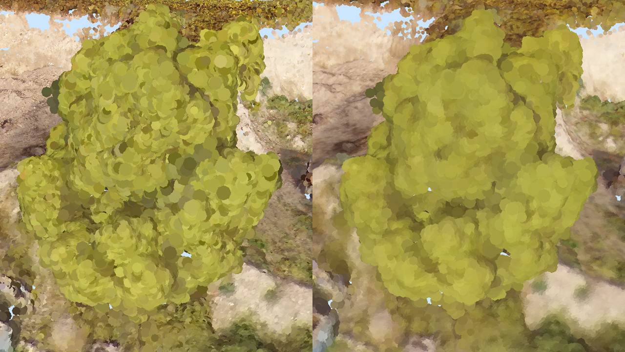
Points with original colours (left) and with blended colours (right)