Generating Vector Graphics

One important point in HOOPS Luminate is that it can be used in a special way to produce non raster outputs. In this tutorial, we’ll start from a simple scene and we’ll generate the edge view of this scene, after an identification and an elimination of all hidden edges from the result. The tutorial will generate edges as a final result, not an image. These edges can be then output for anything requiring vectors and not raster images, such as sending data to postscript files for printing purposes.

Hidden Lines Removal (Raster HLR)

The tutorial starts from a simple scene and replaces it by its view in edges, with hidden edges being identified. It’s important to note that HOOPS Luminate operates at the mesh level: it does not have any knowledge of the topology that was used to generate these meshes (even if in this example we use simple primitives, in the general case, HOOPS Luminate has no topological information available from the source modeling information).

One other important point is that the calculation is made at a given image resolution. The method used calculates image pixels and return analytic information for each pixel. So the vector graphics are generated for a given image resolution and have an accuracy related to the size of a pixel. It’s possible to increase the resolution of the calculation, at the expense of an increased rendering time.

The initial scene and the generated HLR view.

The two extra toolbar buttons in the application can be used to switch back and forth from the normal shaded view of the scene to the HLR view. The HLR view is recalculated and updated each time the button is pressed. After generation, it can be freely moved. We see then that it was created for a given camera and only for that camera.

The Pixel Analysis Callback

The RED::IViewpointRenderList::SetPixelAnalysisCallback method lets any HOOPS Luminate user add a hook on the internal software ray-tracer calculation that occurs during a call to RED::IWindow::FrameTracing. The pixel analysis callback will collect all visible elements that are visible through a pixel from a camera. All collected elements are resulting of analytic intersection between a pixel frustum and geometries that exist in the processed scene. The schema below illustrates the behavior of the pixel analysis callback:

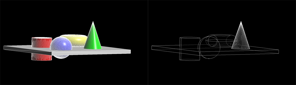
The initial scene and the generated HLR view.

Traditional ray-tracing is not capable of ‘capturing’ the intersection of a volume with geometries because propagated rays have no real volume. Here, we do a processing based on the volume defined by the frustum of a complete pixel. Thanks to the analytic propagation and intersection of this volume with all geometrical primitives found along its path, we’re able to collect all analytic information on the visible data.

The image above illustrates (in red), the shape of a pixel frustum for a perspective camera. The volume is a truncated pyramid, limited by (dnear, dfar) clip limits from the camera eye position. Because intersections are all volumic, the intersection of a geometry element with the volume ends up in a parametric ‘hit interval’ for each primitive that intersects the frustum volume. A ‘t’ parametric value is the raster depth of the considered point as it would appear in a z-buffer. Practically speaking, this is the fragment depth resulting of the model-view-projection transform of the point in space onto the screen for display.

As we can see in the schema, the intersection with an edge results in a (e0, e1) reduced segment that intersects our pyramid volume. The parametric hit interval of this segment is the interval of the two depths of e0 and e1 projected onto screen. In the case of a triangle, the intersection may be more complex, as clipping the triangle against the pyramid volume may result in several intersection points. The callback computes the boundaries of this intersection: the closest point of the intersection between the triangle and the volume from the eye, and the opposite farthest point.

Practically speaking, the pixel analysis callback will be called once:

• For every calculating thread

• For every screen pixel

• For every primitive that intersects the pixel frustum volume

The pixel analysis callback works thanks to the software ray-tracer; therefore, HOOPS Luminate must be started in hybrid or full-software mode for it to work.

Simplification and Parametrization for Dashed Line Display

One problem with the solution displayed at first is that it’s made of thousands of ‘micro’ segments. Each segments stored and returned by the pixel analysis callback was the result of the intersection between an edge in the geometry and a pixel’s frustum pyramid. We need to simplify all this.

The first operation to perform is a RED::ILineShape::Collapse. It’ll merge all duplicate vertices together. This way, we restore a connectivity among all the edges that are displayed. This opens the door for a call to RED::ILineShape::Parametrize. The parametrization operation is a complex connectivity operation that occurs on a set of lines to add parametric length information to all continuous line segments in the shape. The method describes the process in detail in its documentation.

The result of the parametrization is that the shape is transformed into one unique big strip, which is suitable for hardware line stipple. We use a specific parametrization material to ensure the proper display of our result.

Pixel Analysis Callback in Details

Let’s look closely at the callback itself. The first important point is that we need to work on a per-thread basis, as the entire software rendering and analysis process is multi-threaded.

RED::Vector< EdgeData >* evec = ( RED::Vector< EdgeData >* )per_thread_edge_data;

num_thread = rayctx.GetThreadID();

if( num_thread < 0 || num_thread >= (int)evec->size() )
RC_TEST( RED_FAIL );

EdgeData& edata = (*evec)[ num_thread ];

So we have prepared our data beforehand, ensuring that we’ll have one result storage for each calculating thread. The number of threads is identified by RED::IResourceManager::GetNumberOfProcessors.

Then, if we consider the ray in the image below:

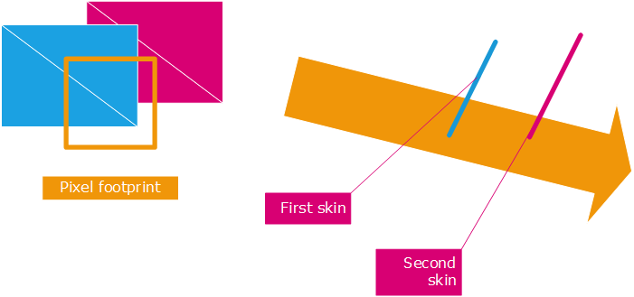
Example of a ray path intersecting primitives

In that example, the ray intersects first the blue set of triangles. The callback will receive 5 datasets: three intersected edges and two triangles. For the purpose of identifying hidden lines, the two first triangles are forming what is called a skin in the callback. This is a connected set of triangles forming a parametric interval. Therefore, in the example above, we have two skins: one formed by blue triangles and one formed by purple triangles. The two are disconnected. Skin identification is performed here in the callback:

if( shape->As< RED::IMeshShape >() )
{
    if( edata._cur_skin_depth == 0.0 )
    {
        // First triangle found: increase our skin depth interval:
        edata._cur_skin_depth = tmax;
    }
    else if( ( edata._cur_skin_depth + 1e-6 ) < tmin )
    {
        // Triangle that is disconnected from the previous triangles depth
        // interval. We consider that our first mesh skin is ended.
        edata._cur_skin_depth = -1.0;
    }
    else if( edata._cur_skin_depth < tmax )
    {
        // Check the heading of our found triangle vs our incoming ray. If barely visible, we consider this as a 'skin break':
        double p0p1[3], p0p2[3], nor[3], len;

        p0p1[0] = p1[0] - p0[0];
        p0p1[1] = p1[1] - p0[1];
        p0p1[2] = p1[2] - p0[2];

        p0p2[0] = p2[0] - p0[0];
        p0p2[1] = p2[1] - p0[1];
        p0p2[2] = p2[2] - p0[2];

        nor[0] = p0p1[1] * p0p2[2] - p0p1[2] * p0p2[1];
        nor[1] = -( p0p1[0] * p0p2[2] - p0p1[2] * p0p2[0] );
        nor[2] = p0p1[0] * p0p2[1] - p0p1[1] - p0p2[0];

        len = nor[0] * nor[0] + nor[1] * nor[1] + nor[2] * nor[2];
        if( abs( len ) > 1e-12 )
        {
        len = 1.0 / sqrt( len );
        nor[0] *= len;
        nor[1] *= len;
        nor[2] *= len;

        if( abs( nor[0] * eye_dir[0] + nor[1] * eye_dir[1] + nor[2] * eye_dir[2] ) > 1e-6 )
        {
            // Increase the depth range of our first mesh skin.
            edata._cur_skin_depth = tmax;
        }
        }
    }
}

We must mention the extra code used to filter triangles nearly perpendicular to the view. These triangles are often met if we render with standard orthographic views (xyz aligned cameras for instance).

Then, any edge which is in the parametric range of a skin is condidered to be visible for that skin (above it). This is what is performed here:

if( edata._cur_skin_depth == 0.0 )
{
    // We haven't met any triangle before us: we're a visible edge.
    depth = 0;
}
else
{
    // If our edge interval is in the range of our first skin depth, we're a
    // visible edge over the first skin triangles. Otherwise, we're a hidden edge.
    depth = ( tmin <= edata._cur_skin_depth ) ? 0 : 1;
}

So this explains the core mechanism of the callback which is based on that identification of visible skins. the process is accurate only at the size of the pixel. False skin continuity can be detected if we have too large pixels (in the example above, this could mean that the blue and purple triangles are considered as one unique skin, so purple edges will appear at depth 0 while they’re hidden). Increasing the resolution will reduce the size of a pixel and increase the whole resulting accuracy.

There are also some other parts in the callback code that we did not detail:

• We filter inner edges: we have prepared our scene with meshes and edges corresponding to meshes. Now among the whole bunch of edges we have, we’re only interested in border edges (that have only one neighbouring triangle) and contour edges (that have one of their triangles facing forward the view and the other facing backward the view). We generally want to discard inner edges. This is the purpose of the test here:

rayctx.Interpolate( nor0, RED::MCL_USER0 );
rayctx.Interpolate( nor1, RED::MCL_USER1 );

len0 = nor0[0] * nor0[0] + nor0[1] * nor0[1] + nor0[2] * nor0[2];
len1 = nor1[0] * nor1[0] + nor1[1] * nor1[1] + nor1[2] * nor1[2];

if( abs( len0 ) < 1e-12 || abs( len1 ) < 1e-12 )
{
    // Border edge case.
    is_edge = true;
}
else
{
    // Inner edge or contour edge case.
    const RED::Matrix* minvtr = rayctx.GetInverseTransposeMatrix();

    if( minvtr )
    {
        minvtr->RotateNormalize( norwcs0, nor0 );
        minvtr->RotateNormalize( norwcs1, nor1 );

        dot0 = norwcs0[0] * eye_dir[0] + norwcs0[1] * eye_dir[1] + norwcs0[2] * eye_dir[2];
        dot1 = norwcs1[0] * eye_dir[0] + norwcs1[1] * eye_dir[1] + norwcs1[2] * eye_dir[2];
    }
    else
    {
        dot0 = nor0[0] * eye_dir[0] + nor0[1] * eye_dir[1] + nor0[2] * eye_dir[2];
        dot1 = nor1[0] * eye_dir[0] + nor1[1] * eye_dir[1] + nor1[2] * eye_dir[2];
    }

    if( dot0 * dot1 < 0.0 )
        is_edge = true;
}

• We clip the found edge to the boundaries of the pixel frustum. This is important, as the visibility information we calculate is only valid for the area covered by our frustum. A single edge may be partly visible and hidden, depending on the geometry layout. This is what is done here:

e0[0] = p0[0]; e0[1] = p0[1]; e0[2] = p0[2]; e0[3] = p0[3];
e1[0] = p1[0]; e1[1] = p1[1]; e1[2] = p1[2]; e1[3] = p1[3];

rayctx.GetPrimaryPixelFrustum( frustum );

for( i = 0, plane = frustum; i < 6; i++, plane += 4 )
{
    dot = plane[0] * ( e1[0] - e0[0] ) +
            plane[1] * ( e1[1] - e0[1] ) +
            plane[2] * ( e1[2] - e0[2] );

    if( dot > 1e-18 || dot < -1e-18 )
    {
        // Intersecting the frustum plane: clip the edge:
        t = -( plane[0] * e0[0] + plane[1] * e0[1] + plane[2] * e0[2] + plane[3] ) / dot;
        if( t > 0.0 && t < 1.0 )
        {
        dot = plane[0] * e0[0] + plane[1] * e0[1] + plane[2] * e0[2] + plane[3];
        if( dot < 0.0 )
        {
            // e0 is on the good side of the plane, cut at e1:
            e1[0] = e0[0] + t * ( e1[0] - e0[0] );
            e1[1] = e0[1] + t * ( e1[1] - e0[1] );
            e1[2] = e0[2] + t * ( e1[2] - e0[2] );
        }
        else
        {
            // e1 is on the good side of the plane, cut at e0:
            e0[0] = e0[0] + t * ( e1[0] - e0[0] );
            e0[1] = e0[1] + t * ( e1[1] - e0[1] );
            e0[2] = e0[2] + t * ( e1[2] - e0[2] );
        }
        }
        else
        {
        // Our segment does not cut the plane, are we on the good side ?
        dot = plane[0] * e0[0] + plane[1] * e0[1] + plane[2] * e0[2] + plane[3];
        if( dot > 0.0 )
            break;
        }
    }
    else
    {
        // Parallel to the frustum plane: on the good or bad side ?
        dot = plane[0] * e0[0] + plane[1] * e0[1] + plane[2] * e0[2] + plane[3];
        if( dot > 0.0 )
        break;
    }
}